
The Reformer - Pushing the limits of language modeling

How the Reformer uses less than 8GB of RAM to train on sequences of half a million tokens
The Reformer model as introduced by Kitaev, Kaiser et al. (2020) is one of the most memory-efficient transformer models for long sequence modeling as of today.
Recently, long sequence modeling has experienced a surge of interest as can be seen by the many submissions from this year alone - Beltagy et al. (2020) , Roy et al. (2020) , Tay et al. , Wang et al. to name a few. The motivation behind long sequence modeling is that many tasks in NLP, e.g. summarization, question answering, require the model to process longer input sequences than models, such as BERT, are able to handle. In tasks that require the model to process a large input sequence, long sequence models do not have to cut the input sequence to avoid memory overflow and thus have been shown to outperform standard "BERT"-like models cf. Beltagy et al. (2020) .
The Reformer pushes the limit of longe sequence modeling by its ability to process up to half a million tokens at once as shown in this demo . As a comparison, a conventional bert-base-uncased model limits the input length to only 512 tokens. In Reformer, each part of the standard transformer architecture is re-engineered to optimize for minimal memory requirement without a significant drop in performance.
The memory improvements can be attributed to 4 features which the Reformer authors introduced to the transformer world:
- Reformer Self-Attention Layer - How to efficiently implement self-attention without being restricted to a local context?
- Chunked Feed Forward Layers - How to get a better time-memory trade-off for large feed forward layers?
- Reversible Residual Layers - How to drastically reduce memory consumption in training by a smart residual architecture?
- Axial Positional Encodings - How to make positional encodings usable for extremely large input sequences?
The goal of this blog post is to give the reader an in-depth understanding of each of the four Reformer features mentioned above. While the explanations are focussed on the Reformer, the reader should get a better intuition under which circumstances each of the four features can be effective for other transformer models as well. The four sections are only loosely connected, so they can very well be read individually.
Reformer is part of the 🤗Transformers library. For all users of the Reformer, it is advised to go through this very detailed blog post to better understand how the model works and how to correctly set its configuration. All equations are accompanied by their equivalent name for the Reformer config, e.g. config.<param_name> , so that the reader can quickly relate to the official docs and configuration file.
Note : Axial Positional Encodings are not explained in the official Reformer paper, but are extensively used in the official codebase. This blog post gives the first in-depth explanation of Axial Positional Encodings.
1. Reformer Self-Attention Layer
Reformer uses two kinds of special self-attention layers: local self-attention layers and Locality Sensitive Hashing ( LSH ) self-attention layers.
To better introduce these new self-attention layers, we will briefly recap conventional self-attention as introduced in Vaswani et al. 2017 .
This blog post uses the same notation and coloring as the popular blog post The illustrated transformer , so the reader is strongly advised to read this blog first.
Important : While Reformer was originally introduced for causal self-attention, it can very well be used for bi-directional self-attention as well. In this post, Reformer's self-attention is presented for bidirectional self-attention.
Recap Global Self-Attention
The core of every Transformer model is the self-attention layer. To recap the conventional self-attention layer, which we refer to here as the global self-attention layer, let us assume we apply a transformer layer on the embedding vector sequence X = x 1 , … , x n \mathbf{X} = \mathbf{x}_1, \ldots, \mathbf{x}_n X = x 1 , … , x n where each vector x i \mathbf{x}_{i} x i is of size config.hidden_size , i.e. d h d_h d h .
In short, a global self-attention layer projects X \mathbf{X} X to the query, key and value matrices Q , K , V \mathbf{Q}, \mathbf{K}, \mathbf{V} Q , K , V and computes the output Z \mathbf{Z} Z using the softmax operation as follows: Z = SelfAttn ( X ) = softmax ( Q K T ) V \mathbf{Z} = \text{SelfAttn}(\mathbf{X}) = \text{softmax}(\mathbf{Q}\mathbf{K}^T) \mathbf{V} Z = SelfAttn ( X ) = softmax ( Q K T ) V with Z \mathbf{Z} Z being of dimension d h × n d_h \times n d h × n (leaving out the key normalization factor and self-attention weights W O \mathbf{W}^{O} W O for simplicity). For more detail on the complete transformer operation, see the illustrated transformer .
Visually, we can illustrate this operation as follows for n = 16 , d h = 3 n=16, d_h=3 n = 16 , d h = 3 :
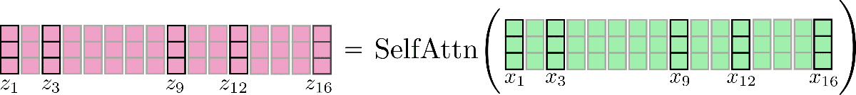
Note that for all visualizations batch_size and config.num_attention_heads is assumed to be 1. Some vectors, e.g. x 3 \mathbf{x_3} x 3 and its corresponding output vector z 3 \mathbf{z_3} z 3 are marked so that LSH self-attention can later be better explained. The presented logic can effortlessly be extended for multi-head self-attention ( config.num_attention_{h}eads > 1). The reader is advised to read the illustrated transformer as a reference for multi-head self-attention.
Important to remember is that for each output vector z i \mathbf{z}_{i} z i , the whole input sequence X \mathbf{X} X is processed. The tensor of the inner dot-product Q K T \mathbf{Q}\mathbf{K}^T Q K T has an asymptotic memory complexity of O ( n 2 ) \mathcal{O}(n^2) O ( n 2 ) which usually represents the memory bottleneck in a transformer model.
This is also the reason why bert-base-cased has a config.max_position_embedding_size of only 512.
Local Self-Attention
Local self-attention is the obvious solution to reducing the O ( n 2 ) \mathcal{O}(n^2) O ( n 2 ) memory bottleneck, allowing us to model longer sequences with a reduced computational cost. In local self-attention the input X = X 1 : n = x 1 , … , x n \mathbf{X} = \mathbf{X}_{1:n} = \mathbf{x}_{1}, \ldots, \mathbf{x}_{n} X = X 1 : n = x 1 , … , x n is cut into n c n_{c} n c chunks: X = [ X 1 : l c , … , X ( n c − 1 ) ∗ l c : n c ∗ l c ] \mathbf{X} = \left[\mathbf{X}_{1:l_{c}}, \ldots, \mathbf{X}_{(n_{c} - 1) * l_{c} : n_{c} * l_{c}}\right] X = [ X 1 : l c , … , X ( n c − 1 ) ∗ l c : n c ∗ l c ] each of length config.local_chunk_length , i.e. l c l_{c} l c , and subsequently global self-attention is applied on each chunk separately.
Let's take our input sequence for n = 16 , d h = 3 n=16, d_h=3 n = 16 , d h = 3 again for visualization:
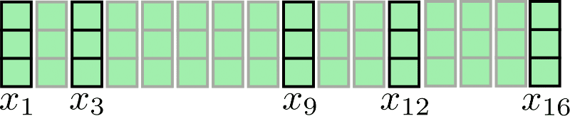
Assuming l c = 4 , n c = 4 l_{c} = 4, n_{c} = 4 l c = 4 , n c = 4 , chunked attention can be illustrated as follows:

As can be seen, the attention operation is applied for each chunk X 1 : 4 , X 5 : 8 , X 9 : 12 , X 13 : 16 \mathbf{X}_{1:4}, \mathbf{X}_{5:8}, \mathbf{X}_{9:12}, \mathbf{X}_{13:16} X 1 : 4 , X 5 : 8 , X 9 : 12 , X 13 : 16 individually. The first drawback of this architecture becomes obvious: Some input vectors have no access to their immediate context, e.g. x 9 \mathbf{x}_9 x 9 has no access to x 8 \mathbf{x}_{8} x 8 and vice-versa in our example. This is problematic because these tokens are not able to learn word representations that take their immediate context into account.
A simple remedy is to augment each chunk with config.local_num_chunks_before , i.e. n p n_{p} n p , chunks and config.local_num_chunks_after , i.e. n a n_{a} n a , so that every input vector has at least access to n p n_{p} n p previous input vectors and n a n_{a} n a following input vectors. This can also be understood as chunking with overlap whereas n p n_{p} n p and n a n_{a} n a define the amount of overlap each chunk has with all previous chunks and following chunks. We denote this extended local self-attention as follows:
Z loc = [ Z 1 : l c loc , … , Z ( n c − 1 ) ∗ l c : n c ∗ l c loc ] , \mathbf{Z}^{\text{loc}} = \left[\mathbf{Z}_{1:l_{c}}^{\text{loc}}, \ldots, \mathbf{Z}_{(n_{c} - 1) * l_{c} : n_{c} * l_{c}}^{\text{loc}}\right], Z loc = [ Z 1 : l c loc , … , Z ( n c − 1 ) ∗ l c : n c ∗ l c loc ] , with Z l c ∗ ( i − 1 ) + 1 : l c ∗ i loc = SelfAttn ( X l c ∗ ( i − 1 − n p ) + 1 : l c ∗ ( i + n a ) ) [ n p ∗ l c : − n a ∗ l c ] , ∀ i ∈ { 1 , … , n c } \mathbf{Z}_{l_{c} * (i - 1) + 1 : l_{c} * i}^{\text{loc}} = \text{SelfAttn}(\mathbf{X}_{l_{c} * (i - 1 - n_{p}) + 1: l_{c} * (i + n_{a})})\left[n_{p} * l_{c}: -n_{a} * l_{c}\right], \forall i \in \{1, \ldots, n_{c} \} Z l c ∗ ( i − 1 ) + 1 : l c ∗ i loc = SelfAttn ( X l c ∗ ( i − 1 − n p ) + 1 : l c ∗ ( i + n a ) ) [ n p ∗ l c : − n a ∗ l c ] , ∀ i ∈ { 1 , … , n c }
Okay, this formula looks quite complicated. Let's make it easier. In Reformer's self-attention layers n a n_{a} n a is usually set to 0 and n p n_{p} n p is set to 1, so let's write down the formula again for i = 1 i = 1 i = 1 :
Z 1 : l c loc = SelfAttn ( X − l c + 1 : l c ) [ l c : ] \mathbf{Z}_{1:l_{c}}^{\text{loc}} = \text{SelfAttn}(\mathbf{X}_{-l_{c} + 1: l_{c}})\left[l_{c}:\right] Z 1 : l c loc = SelfAttn ( X − l c + 1 : l c ) [ l c : ]
We notice that we have a circular relationship so that the first segment can attend the last segment as well. Let's illustrate this slightly enhanced local attention again. First, we apply self-attention within each windowed segment and keep only the central output segment.
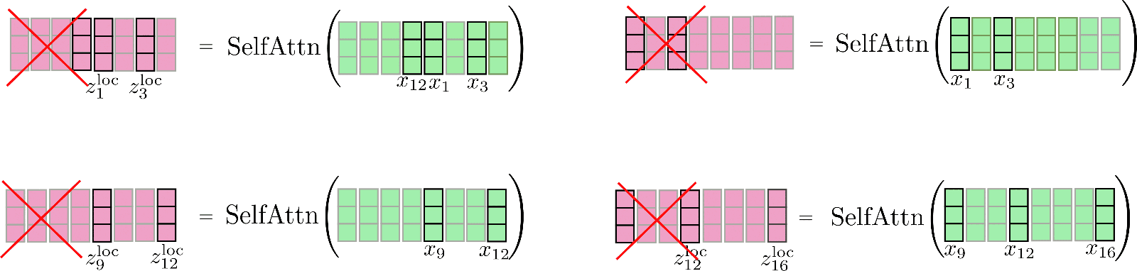
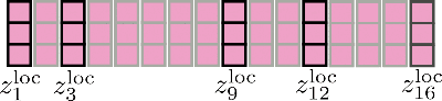
Finally, the relevant output is concatenated to Z loc \mathbf{Z}^{\text{loc}} Z loc and looks as follows.
Note that local self-attention is implemented efficiently way so that no output is computed and subsequently "thrown-out" as shown here for illustration purposes by the red cross.
It's important to note here that extending the input vectors for each chunked self-attention function allows each single output vector z i \mathbf{z}_{i} z i of this self-attention function to learn better vector representations. E.g. each of the output vectors z 5 loc , z 6 loc , z 7 loc , z 8 loc \mathbf{z}_{5}^{\text{loc}}, \mathbf{z}_{6}^{\text{loc}}, \mathbf{z}_{7}^{\text{loc}}, \mathbf{z}_{8}^{\text{loc}} z 5 loc , z 6 loc , z 7 loc , z 8 loc can take into account all of the input vectors X 1 : 8 \mathbf{X}_{1:8} X 1 : 8 to learn better representations.
The gain in memory consumption is quite obvious: The O ( n 2 ) \mathcal{O}(n^2) O ( n 2 ) memory complexity is broken down for each segment individually so that the total asymptotic memory consumption is reduced to O ( n c ∗ l c 2 ) = O ( n ∗ l c ) \mathcal{O}(n_{c} * l_{c}^2) = \mathcal{O}(n * l_{c}) O ( n c ∗ l c 2 ) = O ( n ∗ l c ) .
This enhanced local self-attention is better than the vanilla local self-attention architecture but still has a major drawback in that every input vector can only attend to a local context of predefined size. For NLP tasks that do not require the transformer model to learn long-range dependencies between the input vectors, which include arguably e.g. speech recognition, named entity recognition and causal language modeling of short sentences, this might not be a big issue. Many NLP tasks do require the model to learn long-range dependencies, so that local self-attention could lead to significant performance degradation, e.g.
- Question-answering : the model has to learn the relationship between the question tokens and relevant answer tokens which will most likely not be in the same local range
- Multiple-Choice : the model has to compare multiple answer token segments to each other which are usually separated by a significant length
- Summarization : the model has to learn the relationship between a long sequence of context tokens and a shorter sequence of summary tokens, whereas the relevant relationships between context and summary can most likely not be captured by local self-attention
- etc...
Local self-attention on its own is most likely not sufficient for the transformer model to learn the relevant relationships of input vectors (tokens) to each other.
Therefore, Reformer additionally employs an efficient self-attention layer that approximates global self-attention, called LSH self-attention .
LSH Self-Attention
Alright, now that we have understood how local self-attention works, we can take a stab at the probably most innovative piece of Reformer: Locality sensitive hashing (LSH) Self-Attention .
The premise of LSH self-attention is to be more or less as efficient as local self-attention while approximating global self-attention.
LSH self-attention relies on the LSH algorithm as presented in Andoni et al (2015) , hence its name.
The idea behind LSH self-attention is based on the insight that if n n n is large, the softmax applied on the Q K T \mathbf{Q}\mathbf{K}^T Q K T attention dot-product weights only very few value vectors with values significantly larger than 0 for each query vector.
Let's explain this in more detail. Let k i ∈ K = [ k 1 , … , k n ] T \mathbf{k}_{i} \in \mathbf{K} = \left[\mathbf{k}_1, \ldots, \mathbf{k}_n \right]^T k i ∈ K = [ k 1 , … , k n ] T and q i ∈ Q = [ q 1 , … , q n ] T \mathbf{q}_{i} \in \mathbf{Q} = \left[\mathbf{q}_1, \ldots, \mathbf{q}_n\right]^T q i ∈ Q = [ q 1 , … , q n ] T be the key and query vectors. For each q i \mathbf{q}_{i} q i , the computation softmax ( q i T K T ) \text{softmax}(\mathbf{q}_{i}^T \mathbf{K}^T) softmax ( q i T K T ) can be approximated by using only those key vectors of k j \mathbf{k}_{j} k j that have a high cosine similarity with q i \mathbf{q}_{i} q i . This owes to the fact that the softmax function puts exponentially more weight on larger input values. So far so good, the next problem is to efficiently find the vectors that have a high cosine similarity with q i \mathbf{q}_{i} q i for all i i i .
First, the authors of Reformer notice that sharing the query and key projections: Q = K \mathbf{Q} = \mathbf{K} Q = K does not impact the performance of a transformer model 1 {}^1 1 . Now, instead of having to find the key vectors of high cosine similarity for each query vector q i q_i q i , only the cosine similarity of query vectors to each other has to be found. This is important because there is a transitive property to the query-query vector dot product approximation: If q i \mathbf{q}_{i} q i has a high cosine similarity to the query vectors q j \mathbf{q}_{j} q j and q k \mathbf{q}_{k} q k , then q j \mathbf{q}_{j} q j also has a high cosine similarity to q k \mathbf{q}_{k} q k . Therefore, the query vectors can be clustered into buckets, such that all query vectors that belong to the same bucket have a high cosine similarity to each other. Let's define C m C_{m} C m as the mth set of position indices, such that their corresponding query vectors are in the same bucket: C m = { i ∣ s.t. q i ∈ mth cluster } C_{m} = \{ i | \text{ s.t. } \mathbf{q}_{i} \in \text{mth cluster}\} C m = { i ∣ s.t. q i ∈ mth cluster } and config.num_buckets , i.e. n b n_{b} n b , as the number of buckets.
For each set of indices C m C_{m} C m , the softmax function on the corresponding bucket of query vectors softmax ( Q i ∈ C m Q i ∈ C m T ) \text{softmax}(\mathbf{Q}_{i \in C_{m}} \mathbf{Q}^T_{i \in C_{m}}) softmax ( Q i ∈ C m Q i ∈ C m T ) approximates the softmax function of global self-attention with shared query and key projections softmax ( q i T Q T ) \text{softmax}(\mathbf{q}_{i}^T \mathbf{Q}^T) softmax ( q i T Q T ) for all position indices i i i in C m C_{m} C m .
Second, the authors make use of the LSH algorithm to cluster the query vectors into a predefined number of buckets n b n_{b} n b . The LSH algorithm is an ideal choice here because it is very efficient and is an approximation of the nearest neighbor algorithm for cosine similarity. Explaining the LSH scheme is out-of-scope for this notebook, so let's just keep in mind that for each vector q i \mathbf{q}_{i} q i the LSH algorithm attributes its position index i i i to one of n b n_{b} n b predefined buckets, i.e. LSH ( q i ) = m \text{LSH}(\mathbf{q}_{i}) = m LSH ( q i ) = m with i ∈ { 1 , … , n } i \in \{1, \ldots, n\} i ∈ { 1 , … , n } and m ∈ { 1 , … , n b } m \in \{1, \ldots, n_{b}\} m ∈ { 1 , … , n b } .
Visually, we can illustrate this as follows for our original example:

Third, it can be noted that having clustered all query vectors in n b n_{b} n b buckets, the corresponding set of indices C m C_{m} C m can be used to permute the input vectors x 1 , … , x n \mathbf{x}_1, \ldots, \mathbf{x}_n x 1 , … , x n accordingly 2 {}^2 2 so that shared query-key self-attention can be applied piecewise similar to local attention.
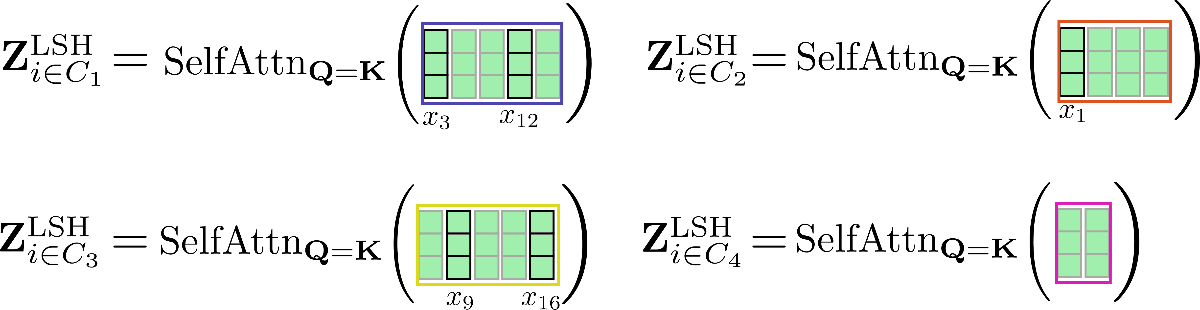
Let's clarify with our example input vectors X = x 1 , . . . , x 16 \mathbf{X} = \mathbf{x}_1, ..., \mathbf{x}_{16} X = x 1 , ... , x 16 and assume config.num_buckets=4 and config.lsh_chunk_length = 4 . Looking at the graphic above we can see that we have assigned each query vector q 1 , … , q 16 \mathbf{q}_1, \ldots, \mathbf{q}_{16} q 1 , … , q 16 to one of the clusters C 1 , C 2 , C 3 , C 4 \mathcal{C}_{1}, \mathcal{C}_{2}, \mathcal{C}_{3}, \mathcal{C}_{4} C 1 , C 2 , C 3 , C 4 . If we now sort the corresponding input vectors x 1 , … , x 16 \mathbf{x}_1, \ldots, \mathbf{x}_{16} x 1 , … , x 16 accordingly, we get the following permuted input X ′ \mathbf{X'} X ′ :

The self-attention mechanism should be applied for each cluster individually so that for each cluster C m \mathcal{C}_m C m the corresponding output is calculated as follows: Z i ∈ C m LSH = SelfAttn Q = K ( X i ∈ C m ) \mathbf{Z}^{\text{LSH}}_{i \in \mathcal{C}_m} = \text{SelfAttn}_{\mathbf{Q}=\mathbf{K}}(\mathbf{X}_{i \in \mathcal{C}_m}) Z i ∈ C m LSH = SelfAttn Q = K ( X i ∈ C m ) .
Let's illustrate this again for our example.
As can be seen, the self-attention function operates on different sizes of matrices, which is suboptimal for efficient batching in GPU and TPU.
To overcome this problem, the permuted input can be chunked the same way it is done for local attention so that each chunk is of size config.lsh_chunk_length . By chunking the permuted input, a bucket might be split into two different chunks. To remedy this problem, in LSH self-attention each chunk attends to its previous chunk config.lsh_num_chunks_before=1 in addition to itself, the same way local self-attention does ( config.lsh_num_chunks_after is usually set to 0). This way, we can be assured that all vectors in a bucket attend to each other with a high probability 3 {}^3 3 .
All in all for all chunks k ∈ { 1 , … , n c } k \in \{1, \ldots, n_{c}\} k ∈ { 1 , … , n c } , LSH self-attention can be noted down as follows:
Z ′ l c ∗ k + 1 : l c ∗ ( k + 1 ) LSH = SelfAttn Q = K ( X ′ l c ∗ k + 1 ) : l c ∗ ( k + 1 ) ) [ l c : ] \mathbf{Z'}_{l_{c} * k + 1:l_{c} * (k + 1)}^{\text{LSH}} = \text{SelfAttn}_{\mathbf{Q} = \mathbf{K}}(\mathbf{X'}_{l_{c} * k + 1): l_{c} * (k + 1)})\left[l_{c}:\right] Z ′ l c ∗ k + 1 : l c ∗ ( k + 1 ) LSH = SelfAttn Q = K ( X ′ l c ∗ k + 1 ) : l c ∗ ( k + 1 ) ) [ l c : ]
with X ′ \mathbf{X'} X ′ and Z ′ \mathbf{Z'} Z ′ being the input and output vectors permuted according to the LSH algorithm. Enough complicated formulas, let's illustrate LSH self-attention.
The permuted vectors X ′ \mathbf{X'} X ′ as shown above are chunked and shared query key self-attention is applied to each chunk.
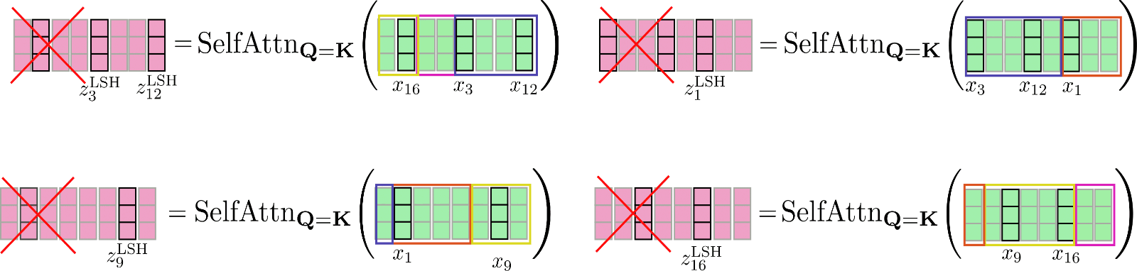
Finally, the output Z ′ LSH \mathbf{Z'}^{\text{LSH}} Z ′ LSH is reordered to its original permutation.

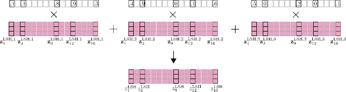
One important feature to mention here as well is that the accuracy of LSH self-attention can be improved by running LSH self-attention config.num_hashes , e.g. n h n_{h} n h times in parallel, each with a different random LSH hash. By setting config.num_hashes > 1 , for each output position i i i , multiple output vectors z i LSH , 1 , … , z i LSH , n h \mathbf{z}^{\text{LSH}, 1}_{i}, \ldots, \mathbf{z}^{\text{LSH}, n_{h}}_{i} z i LSH , 1 , … , z i LSH , n h are computed and subsequently merged: z i LSH = ∑ k n h Z i LSH , k ∗ weight i k \mathbf{z}^{\text{LSH}}_{i} = \sum_k^{n_{h}} \mathbf{Z}^{\text{LSH}, k}_{i} * \text{weight}^k_i z i LSH = ∑ k n h Z i LSH , k ∗ weight i k . The weight i k \text{weight}^k_i weight i k represents the importance of the output vectors z i LSH , k \mathbf{z}^{\text{LSH}, k}_{i} z i LSH , k of hashing round k k k in comparison to the other hashing rounds, and is exponentially proportional to the normalization term of their softmax computation. The intuition behind this is that if the corresponding query vector q i k \mathbf{q}_{i}^{k} q i k have a high cosine similarity with all other query vectors in its respective chunk, then the softmax normalization term of this chunk tends to be high, so that the corresponding output vectors q i k \mathbf{q}_{i}^{k} q i k should be a better approximation to global attention and thus receive more weight than output vectors of hashing rounds with a lower softmax normalization term. For more detail see Appendix A of the paper . For our example, multi-round LSH self-attention can be illustrated as follows.
Great. That's it. Now we know how LSH self-attention works in Reformer.
Regarding the memory complexity, we now have two terms that compete which each other to be the memory bottleneck: the dot-product: O ( n h ∗ n c ∗ l c 2 ) = O ( n ∗ n h ∗ l c ) \mathcal{O}(n_{h} * n_{c} * l_{c}^2) = \mathcal{O}(n * n_{h} * l_{c}) O ( n h ∗ n c ∗ l c 2 ) = O ( n ∗ n h ∗ l c ) and the required memory for LSH bucketing: O ( n ∗ n h ∗ n b 2 ) \mathcal{O}(n * n_{h} * \frac{n_{b}}{2}) O ( n ∗ n h ∗ 2 n b ) with l c l_{c} l c being the chunk length. Because for large n n n , the number of buckets n b 2 \frac{n_{b}}{2} 2 n b grows much faster than the chunk length l c l_{c} l c , the user can again factorize the number of buckets config.num_buckets as explained here .
Let's recap quickly what we have gone through above:
- We want to approximate global attention using the knowledge that the softmax operation only puts significant weights on very few key vectors.
- If key vectors are equal to query vectors this means that for each query vector q i \mathbf{q}_{i} q i , the softmax only puts significant weight on other query vectors that are similar in terms of cosine similarity.
- This relationship works in both ways, meaning if q j \mathbf{q}_{j} q j is similar to q i \mathbf{q}_{i} q i than q j \mathbf{q}_{j} q j is also similar to q i \mathbf{q}_{i} q i , so that we can do a global clustering before applying self-attention on a permuted input.
- We apply local self-attention on the permuted input and re-order the output to its original permutation.
1 {}^{1} 1 The authors run some preliminary experiments confirming that shared query key self-attention performs more or less as well as standard self-attention.
2 {}^{2} 2 To be more exact the query vectors within a bucket are sorted according to their original order. This means if, e.g. the vectors q 1 , q 3 , q 7 \mathbf{q}_1, \mathbf{q}_3, \mathbf{q}_7 q 1 , q 3 , q 7 are all hashed to bucket 2, the order of the vectors in bucket 2 would still be q 1 \mathbf{q}_1 q 1 , followed by q 3 \mathbf{q}_3 q 3 and q 7 \mathbf{q}_7 q 7 .
3 {}^3 3 On a side note, it is to mention the authors put a mask on the query vector q i \mathbf{q}_{i} q i to prevent the vector from attending to itself. Because the cosine similarity of a vector to itself will always be as high or higher than the cosine similarity to other vectors, the query vectors in shared query key self-attention are strongly discouraged to attend to themselves.
Benchmark
Benchmark tools were recently added to Transformers - see here for a more detailed explanation.
To show how much memory can be saved using "local" + "LSH" self-attention, the Reformer model google/reformer-enwik8 is benchmarked for different local_attn_chunk_length and lsh_attn_chunk_length . The default configuration and usage of the google/reformer-enwik8 model can be checked in more detail here .
Let's first do some necessary imports and installs.
#@title Installs and Imports
# pip installs
!pip -qq install git+https://github.com/huggingface/transformers.git
!pip install -qq py3nvml

from transformers import ReformerConfig, PyTorchBenchmark, PyTorchBenchmarkArguments
First, let's benchmark the memory usage of the Reformer model using global self-attention. This can be achieved by setting lsh_attn_chunk_length = local_attn_chunk_length = 8192 so that for all input sequences smaller or equal to 8192, the model automatically switches to global self-attention.
config = ReformerConfig.from_pretrained("google/reformer-enwik8", lsh_attn_chunk_length=16386, local_attn_chunk_length=16386, lsh_num_chunks_before=0, local_num_chunks_before=0)
benchmark_args = PyTorchBenchmarkArguments(sequence_lengths=[2048, 4096, 8192, 16386], batch_sizes=[1], models=["Reformer"], no_speed=True, no_env_print=True)
benchmark = PyTorchBenchmark(configs=[config], args=benchmark_args)
result = benchmark.run()
HBox(children=(FloatProgress(value=0.0, description='Downloading', max=1279.0, style=ProgressStyle(description…
1 / 1
Doesn't fit on GPU. CUDA out of memory. Tried to allocate 2.00 GiB (GPU 0; 11.17 GiB total capacity; 8.87 GiB already allocated; 1.92 GiB free; 8.88 GiB reserved in total by PyTorch)
==================== INFERENCE - MEMORY - RESULT ====================
--------------------------------------------------------------------------------
Model Name Batch Size Seq Length Memory in MB
--------------------------------------------------------------------------------
Reformer 1 2048 1465
Reformer 1 4096 2757
Reformer 1 8192 7893
Reformer 1 16386 N/A
--------------------------------------------------------------------------------The longer the input sequence, the more visible is the quadratic relationship O ( n 2 ) \mathcal{O}(n^2) O ( n 2 ) between input sequence and peak memory usage. As can be seen, in practice it would require a much longer input sequence to clearly observe that doubling the input sequence quadruples the peak memory usage.
For this a google/reformer-enwik8 model using global attention, a sequence length of over 16K results in a memory overflow.
Now, let's activate local and LSH self-attention by using the model's default parameters.
config = ReformerConfig.from_pretrained("google/reformer-enwik8")
  benchmark_args = PyTorchBenchmarkArguments(sequence_lengths=[2048, 4096, 8192, 16384, 32768, 65436], batch_sizes=[1], models=["Reformer"], no_speed=True, no_env_print=True)
  benchmark = PyTorchBenchmark(configs=[config], args=benchmark_args)
  result = benchmark.run()
1 / 1
Doesn't fit on GPU. CUDA out of memory. Tried to allocate 2.00 GiB (GPU 0; 11.17 GiB total capacity; 7.85 GiB already allocated; 1.74 GiB free; 9.06 GiB reserved in total by PyTorch)
Doesn't fit on GPU. CUDA out of memory. Tried to allocate 4.00 GiB (GPU 0; 11.17 GiB total capacity; 6.56 GiB already allocated; 3.99 GiB free; 6.81 GiB reserved in total by PyTorch)
==================== INFERENCE - MEMORY - RESULT ====================
--------------------------------------------------------------------------------
Model Name Batch Size Seq Length Memory in MB
--------------------------------------------------------------------------------
Reformer 1 2048 1785
Reformer 1 4096 2621
Reformer 1 8192 4281
Reformer 1 16384 7607
Reformer 1 32768 N/A
Reformer 1 65436 N/A
--------------------------------------------------------------------------------As expected using local and LSH self-attention is much more memory efficient for longer input sequences, so that the model runs out of memory only at 16K tokens for a 11GB RAM GPU in this notebook.
2. Chunked Feed Forward Layers
Transformer-based models often employ very large feed forward layers after the self-attention layer in parallel. Thereby, this layer can take up a significant amount of the overall memory and sometimes even represent the memory bottleneck of a model. First introduced in the Reformer paper, feed forward chunking is a technique that allows to effectively trade better memory consumption for increased time consumption.
Chunked Feed Forward Layer in Reformer
In Reformer, the LSH - or local self-attention layer is usually followed by a residual connection, which then defines the first part in a transformer block . For more detail on this please refer to this blog .
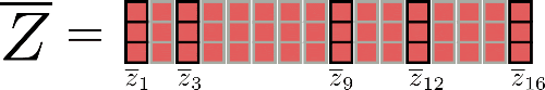
The output of the first part of the transformer block , called normed self-attention output can be written as Z ‾ = Z + X \mathbf{\overline{Z}} = \mathbf{Z} + \mathbf{X} Z = Z + X , with Z \mathbf{Z} Z being either Z LSH \mathbf{Z}^{\text{LSH}} Z LSH or Z loc \mathbf{Z}^\text{loc} Z loc in Reformer.
For our example input x 1 , … , x 16 \mathbf{x}_1, \ldots, \mathbf{x}_{16} x 1 , … , x 16 , we illustrate the normed self-attention output as follows.
Now, the second part of a transformer block usually consists of two feed forward layers 1 ^{1} 1 , defined as Linear int ( … ) \text{Linear}_{\text{int}}(\ldots) Linear int ( … ) that processes Z ‾ \mathbf{\overline{Z}} Z , to an intermediate output Y int \mathbf{Y}_{\text{int}} Y int and Linear out ( … ) \text{Linear}_{\text{out}}(\ldots) Linear out ( … ) that processes the intermediate output to the output Y out \mathbf{Y}_{\text{out}} Y out . The two feed forward layers can be defined by
Y out = Linear out ( Y int ) = Linear out ( Linear int ( Z ‾ ) ) . \mathbf{Y}_{\text{out}} = \text{Linear}_{\text{out}}(\mathbf{Y}_\text{int}) = \text{Linear}_{\text{out}}(\text{Linear}_{\text{int}}(\mathbf{\overline{Z}})). Y out = Linear out ( Y int ) = Linear out ( Linear int ( Z )) .
It is important to remember at this point that mathematically the output of a feed forward layer at position y out , i \mathbf{y}_{\text{out}, i} y out , i only depends on the input at this position y ‾ i \mathbf{\overline{y}}_{i} y i . In contrast to the self-attention layer, every output y out , i \mathbf{y}_{\text{out}, i} y out , i is therefore completely independent of all inputs y ‾ j ≠ i \mathbf{\overline{y}}_{j \ne i} y j = i of different positions.
Let's illustrate the feed forward layers for z ‾ 1 , … , z ‾ 16 \mathbf{\overline{z}}_1, \ldots, \mathbf{\overline{z}}_{16} z 1 , … , z 16 .
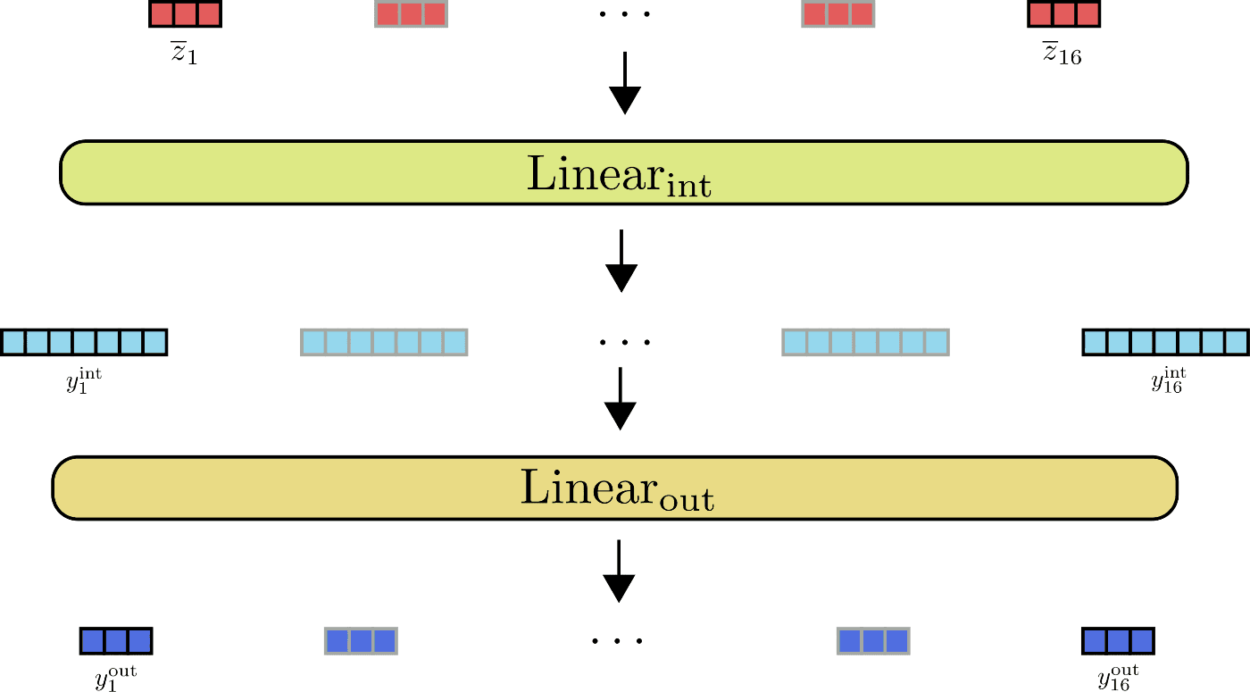
As can be depicted from the illustration, all input vectors z ‾ i \mathbf{\overline{z}}_{i} z i are processed by the same feed forward layer in parallel.
It becomes interesting when one takes a look at the output dimensions of the feed forward layers. In Reformer, the output dimension of Linear int \text{Linear}_{\text{int}} Linear int is defined as config.feed_forward_size , e.g. d f d_{f} d f , and the output dimension of Linear out \text{Linear}_{\text{out}} Linear out is defined as config.hidden_size , i.e. d h d_{h} d h .
The Reformer authors observed that in a transformer model the intermediate dimension d f d_{f} d f usually tends to be much larger than the output dimension 2 ^{2} 2 d h d_{h} d h . This means that the tensor Y int \mathbf{\mathbf{Y}}_\text{int} Y int of dimension d f × n d_{f} \times n d f × n allocates a significant amount of the total memory and can even become the memory bottleneck.
To get a better feeling for the differences in dimensions let's picture the matrices Y int \mathbf{Y}_\text{int} Y int and Y out \mathbf{Y}_\text{out} Y out for our example.
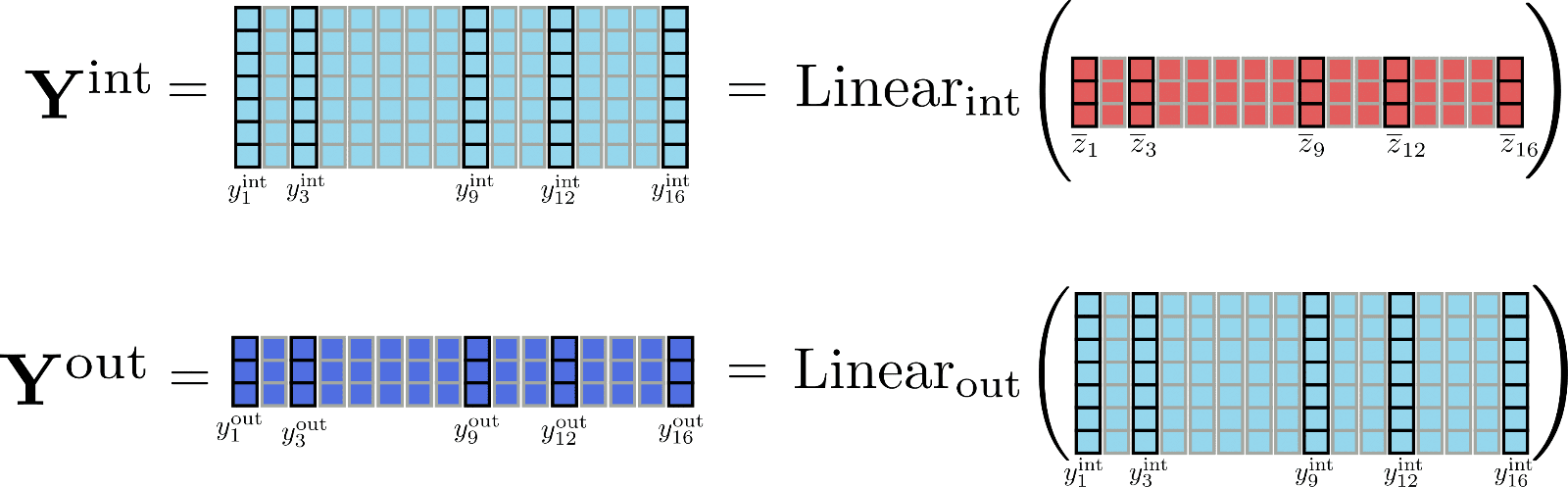
It is becoming quite obvious that the tensor Y int \mathbf{Y}_\text{int} Y int holds much more memory ( d f d h × n \frac{d_{f}}{d_{h}} \times n d h d f × n as much to be exact) than Y out \mathbf{Y}_{\text{out}} Y out . But, is it even necessary to compute the full intermediate matrix Y int \mathbf{Y}_\text{int} Y int ? Not really, because relevant is only the output matrix Y out \mathbf{Y}_\text{out} Y out . To trade memory for speed, one can thus chunk the linear layers computation to only process one chunk at the time. Defining config.chunk_size_feed_forward as c f c_{f} c f , chunked linear layers are defined as Y out = [ Y out , 1 : c f , … , Y out , ( n − c f ) : n ] \mathbf{Y}_{\text{out}} = \left[\mathbf{Y}_{\text{out}, 1: c_{f}}, \ldots, \mathbf{Y}_{\text{out}, (n - c_{f}): n}\right] Y out = [ Y out , 1 : c f , … , Y out , ( n − c f ) : n ] with Y out , ( c f ∗ i ) : ( i ∗ c f + i ) = Linear out ( Linear int ( Z ‾ ( c f ∗ i ) : ( i ∗ c f + i ) ) ) \mathbf{Y}_{\text{out}, (c_{f} * i): (i * c_{f} + i)} = \text{Linear}_{\text{out}}(\text{Linear}_{\text{int}}(\mathbf{\overline{Z}}_{(c_{f} * i): (i * c_{f} + i)})) Y out , ( c f ∗ i ) : ( i ∗ c f + i ) = Linear out ( Linear int ( Z ( c f ∗ i ) : ( i ∗ c f + i ) )) . In practice, it just means that the output is incrementally computed and concatenated to avoid having to store the whole intermediate tensor Y int \mathbf{Y}_{\text{int}} Y int in memory.
Assuming c f = 1 c_{f}=1 c f = 1 for our example we can illustrate the incremental computation of the output for position i = 9 i=9 i = 9 as follows.
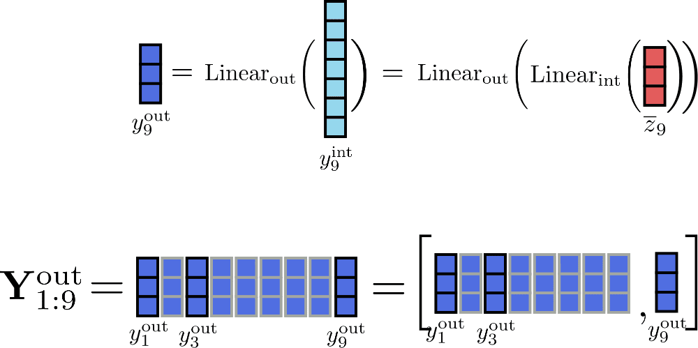
By processing the inputs in chunks of size 1, the only tensors that have to be stored in memory at the same time are Y out \mathbf{Y}_\text{out} Y out of a maximum size of 16 × d h 16 \times d_{h} 16 × d h , y int , i \mathbf{y}_{\text{int}, i} y int , i of size d f d_{f} d f and the input Z ‾ \mathbf{\overline{Z}} Z of size 16 × d h 16 \times d_{h} 16 × d h , with d h d_{h} d h being config.hidden_size 3 ^{3} 3 .
Finally, it is important to remember that chunked linear layers yield a mathematically equivalent output to conventional linear layers and can therefore be applied to all transformer linear layers. Making use of config.chunk_size_feed_forward therefore allows a better trade-off between memory and speed in certain use cases.
1 {}^1 1 For a simpler explanation, the layer norm layer which is normally applied to Z ‾ \mathbf{\overline{Z}} Z before being processed by the feed forward layers is omitted for now.
2 {}^2 2 In bert-base-uncased , e.g. the intermediate dimension d f d_{f} d f is with 3072 four times larger than the output dimension d h d_{h} d h .
3 {}^3 3 As a reminder, the output config.num_attention_heads is assumed to be 1 for the sake of clarity and illustration in this notebook, so that the output of the self-attention layers can be assumed to be of size config.hidden_size .
More information on chunked linear / feed forward layers can also be found here on the 🤗Transformers docs.
Benchmark
Let's test how much memory can be saved by using chunked feed forward layers.
#@title Installs and Imports
# pip installs
!pip -qq install git+https://github.com/huggingface/transformers.git
!pip install -qq py3nvml

from transformers import ReformerConfig, PyTorchBenchmark, PyTorchBenchmarkArguments
Building wheel for transformers (setup.py) ... [?25l[?25hdoneFirst, let's compare the default google/reformer-enwik8 model without chunked feed forward layers to the one with chunked feed forward layers.
config_no_chunk = ReformerConfig.from_pretrained("google/reformer-enwik8")  # no chunk
config_chunk = ReformerConfig.from_pretrained("google/reformer-enwik8", chunk_size_feed_forward=1)  # feed forward chunk
benchmark_args = PyTorchBenchmarkArguments(sequence_lengths=[1024, 2048, 4096], batch_sizes=[8], models=["Reformer-No-Chunk", "Reformer-Chunk"], no_speed=True, no_env_print=True)
benchmark = PyTorchBenchmark(configs=[config_no_chunk, config_chunk], args=benchmark_args)
result = benchmark.run()
1 / 2
Doesn't fit on GPU. CUDA out of memory. Tried to allocate 2.00 GiB (GPU 0; 11.17 GiB total capacity; 7.85 GiB already allocated; 1.74 GiB free; 9.06 GiB reserved in total by PyTorch)
2 / 2
Doesn't fit on GPU. CUDA out of memory. Tried to allocate 2.00 GiB (GPU 0; 11.17 GiB total capacity; 7.85 GiB already allocated; 1.24 GiB free; 9.56 GiB reserved in total by PyTorch)
==================== INFERENCE - MEMORY - RESULT ====================
--------------------------------------------------------------------------------
Model Name Batch Size Seq Length Memory in MB
--------------------------------------------------------------------------------
Reformer-No-Chunk 8 1024 4281
Reformer-No-Chunk 8 2048 7607
Reformer-No-Chunk 8 4096 N/A
Reformer-Chunk 8 1024 4309
Reformer-Chunk 8 2048 7669
Reformer-Chunk 8 4096 N/A
--------------------------------------------------------------------------------Interesting, chunked feed forward layers do not seem to help here at all. The reason is that config.feed_forward_size is not sufficiently large to make a real difference. Only at longer sequence lengths of 4096, a slight decrease in memory usage can be seen.
Let's see what happens to the memory peak usage if we increase the size of the feed forward layer by a factor of 4 and reduce the number of attention heads also by a factor of 4 so that the feed forward layer becomes the memory bottleneck.
config_no_chunk = ReformerConfig.from_pretrained("google/reformer-enwik8", chunk_size_feed_forward=0, num_attention_{h}eads=2, feed_forward_size=16384)  # no chuck
config_chunk = ReformerConfig.from_pretrained("google/reformer-enwik8", chunk_size_feed_forward=1, num_attention_{h}eads=2, feed_forward_size=16384)  # feed forward chunk
benchmark_args = PyTorchBenchmarkArguments(sequence_lengths=[1024, 2048, 4096], batch_sizes=[8], models=["Reformer-No-Chunk", "Reformer-Chunk"], no_speed=True, no_env_print=True)
benchmark = PyTorchBenchmark(configs=[config_no_chunk, config_chunk], args=benchmark_args)
result = benchmark.run()
1 / 2
2 / 2
==================== INFERENCE - MEMORY - RESULT ====================
--------------------------------------------------------------------------------
Model Name Batch Size Seq Length Memory in MB
--------------------------------------------------------------------------------
Reformer-No-Chunk 8 1024 3743
Reformer-No-Chunk 8 2048 5539
Reformer-No-Chunk 8 4096 9087
Reformer-Chunk 8 1024 2973
Reformer-Chunk 8 2048 3999
Reformer-Chunk 8 4096 6011
--------------------------------------------------------------------------------Now a clear decrease in peak memory usage can be seen for longer input sequences. As a conclusion, it should be noted chunked feed forward layers only makes sense for models having few attention heads and large feed forward layers.
3. Reversible Residual Layers
Reversible residual layers were first introduced in N. Gomez et al and used to reduce memory consumption when training the popular ResNet model. Mathematically, reversible residual layers are slightly different to "real" residual layers but do not require the activations to be saved during the forward pass, which can drastically reduce memory consumption for training.
Reversible Residual Layers in Reformer
Let's start by investigating why training a model requires much more memory than the inference of the model.
When running a model in inference, the required memory equals more or less the memory it takes to compute the single largest tensor in the model. On the other hand, when training a model, the required memory equals more or less the sum of all differentiable tensors.
This is not surprising when considering how auto differentiation works in deep learning frameworks. These lecture slides by Roger Grosse of the University of Toronto are great to better understand auto differentiation.