Leveraging Pre-trained Language Model Checkpoints for Encoder-Decoder Models

Leveraging Pre-trained Language Model Checkpoints for Encoder-Decoder Models

• +10

Transformer-based encoder-decoder models were proposed in Vaswani et al. (2017) and have recently experienced a surge of interest, e.g. Lewis et al. (2019) , Raffel et al. (2019) , Zhang et al. (2020) , Zaheer et al. (2020) , Yan et al. (2020) .

Similar to BERT and GPT2, massive pre-trained encoder-decoder models have shown to significantly boost performance on a variety of sequence-to-sequence tasks Lewis et al. (2019) , Raffel et al. (2019) . However, due to the enormous computational cost attached to pre-training encoder-decoder models, the development of such models is mainly limited to large companies and institutes.

In Leveraging Pre-trained Checkpoints for Sequence Generation Tasks (2020) , Sascha Rothe, Shashi Narayan and Aliaksei Severyn initialize encoder-decoder model with pre-trained encoder and/or decoder-only checkpoints ( e.g. BERT, GPT2) to skip the costly pre-training. The authors show that such warm-started encoder-decoder models yield competitive results to large pre-trained encoder-decoder models, such as T5 , and Pegasus on multiple sequence-to-sequence tasks at a fraction of the training cost.

In this notebook, we will explain in detail how encoder-decoder models can be warm-started, give practical tips based on Rothe et al. (2020) , and finally go over a complete code example showing how to warm-start encoder-decoder models with 🤗Transformers.

This notebook is divided into 4 parts:

• Introduction - Short summary of pre-trained language models in NLP and the need for warm-starting encoder-decoder models.
• Warm-starting encoder-decoder models (Theory) - Illustrative explanation on how encoder-decoder models are warm-started?
• Warm-starting encoder-decoder models (Analysis) - Summary of Leveraging Pre-trained Checkpoints for Sequence Generation Tasks (2020) - What model combinations are effective to warm-start encoder-decoder models; How does it differ from task to task?
• Warm-starting encoder-decoder models with 🤗Transformers (Practice) - Complete code example showcasing in-detail how to use the EncoderDecoderModel framework to warm-start transformer-based encoder-decoder models.

It is highly recommended (probably even necessary) to have read this blog post about transformer-based encoder-decoder models.

Let's start by giving some back-ground on warm-starting encoder-decoder models.

Introduction

Recently, pre-trained language models 1 {}^1 1 have revolutionized the field of natural language processing (NLP).

The first pre-trained language models were based on recurrent neural networks (RNN) as proposed Dai et al. (2015) . Dai et. al showed that pre-training an RNN-based model on unlabelled data and subsequently fine-tuning 2 {}^2 2 it on a specific task yields better results than training a randomly initialized model directly on such a task. However, it was only in 2018, when pre-trained language models become widely accepted in NLP. ELMO by Peters et al. and ULMFit by Howard et al. were the first pre-trained language model to significantly improve the state-of-the-art on an array of natural language understanding (NLU) tasks. Just a couple of months later, OpenAI and Google published transformer-based pre-trained language models, called GPT by Radford et al. and BERT by Devlin et al. respectively. The improved efficiency of transformer-based language models over RNNs allowed GPT2 and BERT to be pre-trained on massive amounts of unlabeled text data. Once pre-trained, BERT and GPT were shown to require very little fine-tuning to shatter state-of-art results on more than a dozen NLU tasks 3 {}^3 3 .

The capability of pre-trained language models to effectively transfer task-agnostic knowledge to task-specific knowledge turned out to be a great catalyst for NLU. Whereas engineers and researchers previously had to train a language model from scratch, now publicly available checkpoints of large pre-trained language models can be fine-tuned at a fraction of the cost and time. This can save millions in industry and allows for faster prototyping and better benchmarks in research.

Pre-trained language models have established a new level of performance on NLU tasks and more and more research has been built upon leveraging such pre-trained language models for improved NLU systems. However, standalone BERT and GPT models have been less successful for sequence-to-sequence tasks, e.g. text-summarization , machine translation , sentence-rephrasing , etc.

Sequence-to-sequence tasks are defined as a mapping from an input sequence X 1 : n \mathbf{X}_{1:n} X 1 : n ​ to an output sequence Y 1 : m \mathbf{Y}_{1:m} Y 1 : m ​ of a-priori unknown output length m m m . Hence, a sequence-to-sequence model should define the conditional probability distribution of the output sequence Y 1 : m \mathbf{Y}_{1:m} Y 1 : m ​ conditioned on the input sequence X 1 : n \mathbf{X}_{1:n} X 1 : n ​ :

p θ model ( Y 1 : m ∣ X 1 : n ) . p_{\theta_{\text{model}}}(\mathbf{Y}_{1:m} | \mathbf{X}_{1:n}). p θ model ​ ​ ( Y 1 : m ​ ∣ X 1 : n ​ ) .

Without loss of generality, an input word sequence of n n n words is hereby represented by the vector sequnece X 1 : n = x 1 , … , x n \mathbf{X}_{1:n} = \mathbf{x}_1, \ldots, \mathbf{x}_n X 1 : n ​ = x 1 ​ , … , x n ​ and an output sequence of m m m words as Y 1 : m = y 1 , … , y m \mathbf{Y}_{1:m} = \mathbf{y}_1, \ldots, \mathbf{y}_m Y 1 : m ​ = y 1 ​ , … , y m ​ .

Let's see how BERT and GPT2 would be fit to model sequence-to-sequence tasks.

BERT

BERT is an encoder-only model, which maps an input sequence X 1 : n \mathbf{X}_{1:n} X 1 : n ​ to a contextualized encoded sequence X ‾ 1 : n \mathbf{\overline{X}}_{1:n} X 1 : n ​ :

f θ BERT : X 1 : n → X ‾ 1 : n . f_{\theta_{\text{BERT}}}: \mathbf{X}_{1:n} \to \mathbf{\overline{X}}_{1:n}. f θ BERT ​ ​ : X 1 : n ​ → X 1 : n ​ .

BERT's contextualized encoded sequence X ‾ 1 : n \mathbf{\overline{X}}_{1:n} X 1 : n ​ can then further be processed by a classification layer for NLU classification tasks, such as sentiment analysis , natural language inference , etc. To do so, the classification layer, i.e. typically a pooling layer followed by a feed-forward layer, is added as a final layer on top of BERT to map the contextualized encoded sequence X ‾ 1 : n \mathbf{\overline{X}}_{1:n} X 1 : n ​ to a class c c c :

f θ p,c : X ‾ 1 : n → c . f_{\theta{\text{p,c}}}: \mathbf{\overline{X}}_{1:n} \to c. f θ p,c ​ : X 1 : n ​ → c .

It has been shown that adding a pooling- and classification layer, defined as θ p,c \theta_{\text{p,c}} θ p,c ​ , on top of a pre-trained BERT model θ BERT \theta_{\text{BERT}} θ BERT ​ and subsequently fine-tuning the complete model { θ p,c , θ BERT } \{\theta_{\text{p,c}}, \theta_{\text{BERT}}\} { θ p,c ​ , θ BERT ​ } can yield state-of-the-art performances on a variety of NLU tasks, cf. to BERT by Devlin et al. .

Let's visualize BERT.

The BERT model is shown in grey. The model stacks multiple BERT blocks , each of which is composed of bi-directional self-attention layers (shown in the lower part of the red box) and two feed-forward layers (short in the upper part of the red box).

Each BERT block makes use of bi-directional self-attention to process an input sequence x ′ 1 , … , x ′ n \mathbf{x'}_1, \ldots, \mathbf{x'}_n x ′ 1 ​ , … , x ′ n ​ (shown in light grey) to a more "refined" contextualized output sequence x ′ ′ 1 , … , x ′ ′ n \mathbf{x''}_1, \ldots, \mathbf{x''}_n x ′′ 1 ​ , … , x ′′ n ​ (shown in slightly darker grey) 4 {}^4 4 . The contextualized output sequence of the final BERT block, i.e. X ‾ 1 : n \mathbf{\overline{X}}_{1:n} X 1 : n ​ , can then be mapped to a single output class c c c by adding a task-specific classification layer (shown in orange) as explained above.

Encoder-only models can only map an input sequence to an output sequence of a priori known output length. In conclusion, the output dimension does not depend on the input sequence, which makes it disadvantageous and impractical to use encoder-only models for sequence-to-sequence tasks.

As for all encoder-only models, BERT's architecture corresponds exactly to the architecture of the encoder part of transformer-based encoder-decoder models as shown in the "Encoder" section in the Encoder-Decoder notebook .

GPT2

GPT2 is a decoder-only model, which makes use of uni-directional ( i.e. "causal") self-attention to define a mapping from an input sequence Y 0 : m − 1 \mathbf{Y}_{0: m - 1} Y 0 : m − 1 ​ 1 {}^1 1 to a "next-word" logit vector sequence L 1 : m \mathbf{L}_{1:m} L 1 : m ​ :

f θ GPT2 : Y 0 : m − 1 → L 1 : m . f_{\theta_{\text{GPT2}}}: \mathbf{Y}_{0: m - 1} \to \mathbf{L}_{1:m}. f θ GPT2 ​ ​ : Y 0 : m − 1 ​ → L 1 : m ​ .

By processing the logit vectors L 1 : m \mathbf{L}_{1:m} L 1 : m ​ with the softmax operation, the model can define the probability distribution of the word sequence Y 1 : m \mathbf{Y}_{1:m} Y 1 : m ​ . To be exact, the probability distribution of the word sequence Y 1 : m \mathbf{Y}_{1:m} Y 1 : m ​ can be factorized into m − 1 m-1 m − 1 conditional "next word" distributions:

p θ GPT2 ( Y 1 : m ) = ∏ i = 1 m p θ GPT2 ( y i ∣ Y 0 : i − 1 ) . p_{\theta_{\text{GPT2}}}(\mathbf{Y}_{1:m}) = \prod_{i=1}^{m} p_{\theta_{\text{GPT2}}}(\mathbf{y}_i | \mathbf{Y}_{0:i-1}). p θ GPT2 ​ ​ ( Y 1 : m ​ ) = i = 1 ∏ m ​ p θ GPT2 ​ ​ ( y i ​ ∣ Y 0 : i − 1 ​ ) . p θ GPT2 ( y i ∣ Y 0 : i − 1 ) p_{\theta_{\text{GPT2}}}(\mathbf{y}_i | \mathbf{Y}_{0:i-1}) p θ GPT2 ​ ​ ( y i ​ ∣ Y 0 : i − 1 ​ ) hereby presents the probability distribution of the next word y i \mathbf{y}_i y i ​ given all previous words y 0 , … , y i − 1 \mathbf{y}_0, \ldots, \mathbf{y}_{i-1} y 0 ​ , … , y i − 1 ​ 3 {}^3 3 and is defined as the softmax operation applied on the logit vector l i \mathbf{l}_i l i ​ . To summarize, the following equations hold true.

p θ gpt2 ( y i ∣ Y 0 : i − 1 ) = Softmax ( l i ) = Softmax ( f θ GPT2 ( Y 0 : i − 1 ) ) . p_{\theta_{\text{gpt2}}}(\mathbf{y}_i | \mathbf{Y}_{0:i-1}) = \textbf{Softmax}(\mathbf{l}_i) = \textbf{Softmax}(f_{\theta_{\text{GPT2}}}(\mathbf{Y}_{0: i - 1})). p θ gpt2 ​ ​ ( y i ​ ∣ Y 0 : i − 1 ​ ) = Softmax ( l i ​ ) = Softmax ( f θ GPT2 ​ ​ ( Y 0 : i − 1 ​ )) .

For more detail, please refer to the decoder section of the encoder-decoder blog post.

Let's visualize GPT2 now as well.

Analogous to BERT, GPT2 is composed of a stack of GPT2 blocks . In contrast to BERT block, GPT2 block makes use of uni-directional self-attention to process some input vectors y ′ 0 , … , y ′ m − 1 \mathbf{y'}_0, \ldots, \mathbf{y'}_{m-1} y ′ 0 ​ , … , y ′ m − 1 ​ (shown in light blue on the bottom right) to an output vector sequence y ′ ′ 0 , … , y ′ ′ m − 1 \mathbf{y''}_0, \ldots, \mathbf{y''}_{m-1} y ′′ 0 ​ , … , y ′′ m − 1 ​ (shown in darker blue on the top right). In addition to the GPT2 block stack, the model also has a linear layer, called LM Head , which maps the output vectors of the final GPT2 block to the logit vectors l 1 , … , l m \mathbf{l}_1, \ldots, \mathbf{l}_m l 1 ​ , … , l m ​ . As mentioned earlier, a logit vector l i \mathbf{l}_i l i ​ can then be used to sample of new input vector y i \mathbf{y}_i y i ​ 5 {}^5 5 .

GPT2 is mainly used for open-domain text generation. First, an input prompt Y 0 : i − 1 \mathbf{Y}_{0:i-1} Y 0 : i − 1 ​ is fed to the model to yield the conditional distribution p θ gpt2 ( y ∣ Y 0 : i − 1 ) p_{\theta_{\text{gpt2}}}(\mathbf{y} | \mathbf{Y}_{0:i-1}) p θ gpt2 ​ ​ ( y ∣ Y 0 : i − 1 ​ ) . Then the next word y i \mathbf{y}_i y i ​ is sampled from the distribution (represented by the grey arrows in the graph above) and consequently append to the input. In an auto-regressive fashion the word y i + 1 \mathbf{y}_{i+1} y i + 1 ​ can then be sampled from p θ gpt2 ( y ∣ Y 0 : i ) p_{\theta_{\text{gpt2}}}(\mathbf{y} | \mathbf{Y}_{0:i}) p θ gpt2 ​ ​ ( y ∣ Y 0 : i ​ ) and so on.

GPT2 is therefore well-suited for language generation , but less so for conditional generation. By setting the input prompt Y 0 : i − 1 \mathbf{Y}_{0: i-1} Y 0 : i − 1 ​ equal to the sequence input X 1 : n \mathbf{X}_{1:n} X 1 : n ​ , GPT2 can very well be used for conditional generation. However, the model architecture has a fundamental drawback compared to the encoder-decoder architecture as explained in Raffel et al. (2019) on page 17. In short, uni-directional self-attention forces the model's representation of the sequence input X 1 : n \mathbf{X}_{1:n} X 1 : n ​ to be unnecessarily limited since x i \mathbf{x}_i x i ​ cannot depend on x i + 1 , ∀ i ∈ { 1 , … , n } \mathbf{x}_{i+1}, \forall i \in \{1,\ldots, n\} x i + 1 ​ , ∀ i ∈ { 1 , … , n } .

Encoder-Decoder

Because encoder-only models require to know the output length a priori , they seem unfit for sequence-to-sequence tasks. Decoder-only models can function well for sequence-to-sequence tasks, but also have certain architectural limitations as explained above.

The current predominant approach to tackle sequence-to-sequence tasks are transformer-based encoder-decoder models - often also called seq2seq transformer models. Encoder-decoder models were introduced in Vaswani et al. (2017) and since then have been shown to perform better on sequence-to-sequence tasks than stand-alone language models ( i.e. decoder-only models), e.g. Raffel et al. (2020) . In essence, an encoder-decoder model is the combination of a stand-alone encoder, such as BERT, and a stand-alone decoder model, such as GPT2. For more details on the exact architecture of transformer-based encoder-decoder models, please refer to this blog post .

Now, we know that freely available checkpoints of large pre-trained stand-alone encoder and decoder models, such as BERT and GPT , can boost performance and reduce training cost for many NLU tasks, We also know that encoder-decoder models are essentially the combination of stand-alone encoder and decoder models. This naturally brings up the question of how one can leverage stand-alone model checkpoints for encoder-decoder models and which model combinations are most performant on certain sequence-to-sequence tasks.

In 2020, Sascha Rothe, Shashi Narayan, and Aliaksei Severyn investigated exactly this question in their paper Leveraging Pre-trained Checkpoints for Sequence Generation Tasks . The paper offers a great analysis of different encoder-decoder model combinations and fine-tuning techniques, which we will study in more detail later.

Composing an encoder-decoder model of pre-trained stand-alone model checkpoints is defined as warm-starting the encoder-decoder model. The following sections show how warm-starting an encoder-decoder model works in theory, how one can put the theory into practice with 🤗Transformers, and also gives practical tips for better performance.

1 {}^1 1 A pre-trained language model is defined as a neural network:

• that has been trained on unlabeled text data, i.e. in a task-agnostic, unsupervised fashion, and
• that processes a sequence of input words into a context-dependent embedding. E.g. the continuous bag-of-words and skip-gram model from Mikolov et al. (2013) is not considered a pre-trained language model because the embeddings are context-agnostic.

2 {}^2 2 Fine-tuning is defined as the task-specific training of a model that has been initialized with the weights of a pre-trained language model.

3 {}^3 3 The input vector y 0 \mathbf{y}_0 y 0 ​ corresponds hereby to the BOS \text{BOS} BOS embedding vector required to predict the very first output word y 1 \mathbf{y}_1 y 1 ​ .

4 {}^4 4 Without loss of generalitiy, we exclude the normalization layers to not clutter the equations and illustrations.

5 {}^5 5 For more detail on why uni-directional self-attention is used for "decoder-only" models, such as GPT2, and how sampling works exactly, please refer to the decoder section of the encoder-decoder blog post.

Warm-starting encoder-decoder models (Theory)

Having read the introduction, we are now familiar with encoder-only - and decoder-only models. We have noticed that the encoder-decoder model architecture is essentially a composition of a stand-alone encoder model and a stand-alone decoder model, which led us to the question of how one can warm-start encoder-decoder models from stand-alone model checkpoints.

There are multiple possibilities to warm-start an encoder-decoder model. One can

1. initialize both the encoder and decoder part from an encoder-only model checkpoint, e.g. BERT,
2. initialize the encoder part from an encoder-only model checkpoint, e.g. BERT, and the decoder part from and a decoder-only checkpoint, e.g. GPT2,
3. initialize only the encoder part with an encoder-only model checkpoint, or
4. initialize only the decoder part with a decoder-only model checkpoint.

In the following, we will put the focus on possibilities 1. and 2. Possibilities 3. and 4. are trivial after having understood the first two.

Recap Encoder-Decoder Model

First, let's do a quick recap of the encoder-decoder architecture.

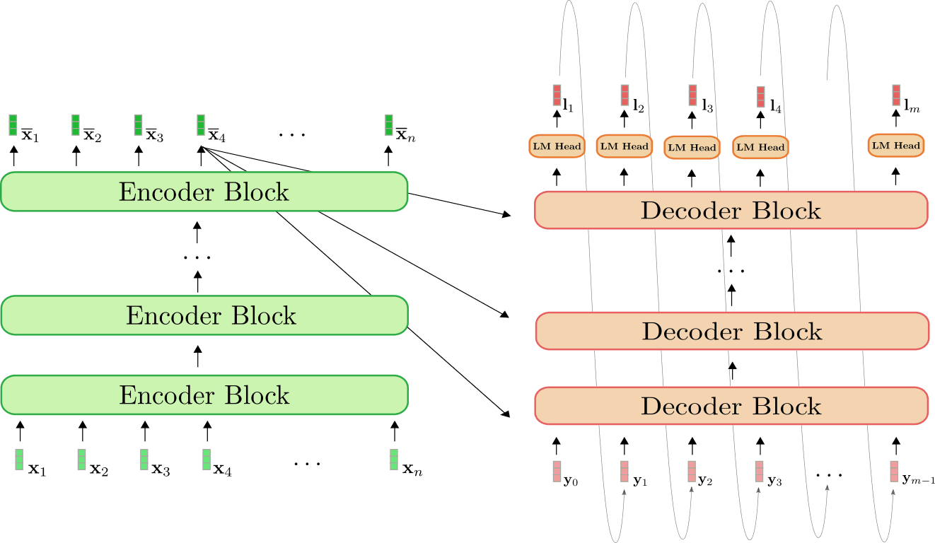
The encoder (shown in green) is a stack of encoder blocks . Each encoder block is composed of a bi-directional self-attention layer, and two feed-forward layers 1 {}^1 1 . The decoder (shown in orange) is a stack of decoder blocks , followed by a dense layer, called LM Head . Each decoder block is composed of a uni-directional self-attention layer, a cross-attention layer, and two feed-forward layers.

The encoder maps the input sequence X 1 : n \mathbf{X}_{1:n} X 1 : n ​ to a contextualized encoded sequence X ‾ 1 : n \mathbf{\overline{X}}_{1:n} X 1 : n ​ in the exact same way BERT does. The decoder then maps the contextualized encoded sequence X ‾ 1 : n \mathbf{\overline{X}}_{1:n} X 1 : n ​ and a target sequence Y 0 : m − 1 \mathbf{Y}_{0:m-1} Y 0 : m − 1 ​ to the logit vectors L 1 : m \mathbf{L}_{1:m} L 1 : m ​ . Analogous to GPT2, the logits are then used to define the distribution of the target sequence Y 1 : m \mathbf{Y}_{1:m} Y 1 : m ​ conditioned on the input sequence X 1 : n \mathbf{X}_{1:n} X 1 : n ​ by means of a softmax operation.

To put it into mathematical terms, first, the conditional distribution is factorized into m − 1 m - 1 m − 1 conditional distributions of the next word y i \mathbf{y}_i y i ​ by Bayes' rule.

p θ enc, dec ( Y 1 : m ∣ X 1 : n ) = p θ dec ( Y 1 : m ∣ X ‾ 1 : n ) = ∏ i = 1 m p θ dec ( y i ∣ Y 0 : i − 1 , X ‾ 1 : n ) , with X ‾ 1 : n = f θ enc ( X 1 : n ) . p_{\theta_{\text{enc, dec}}}(\mathbf{Y}_{1:m} | \mathbf{X}_{1:n}) = p_{\theta_{\text{dec}}}(\mathbf{Y}_{1:m} | \mathbf{\overline{X}}_{1:n}) = \prod_{i=1}^m p_{\theta_{\text{dec}}}(\mathbf{y}_i | \mathbf{Y}_{0: i -1}, \mathbf{\overline{X}}_{1:n}), \text{ with } \mathbf{\overline{X}}_{1:n} = f_{\theta_{\text{enc}}}(\mathbf{X}_{1:n}). p θ enc, dec ​ ​ ( Y 1 : m ​ ∣ X 1 : n ​ ) = p θ dec ​ ​ ( Y 1 : m ​ ∣ X 1 : n ​ ) = i = 1 ∏ m ​ p θ dec ​ ​ ( y i ​ ∣ Y 0 : i − 1 ​ , X 1 : n ​ ) , with X 1 : n ​ = f θ enc ​ ​ ( X 1 : n ​ ) .

Each "next-word" conditional distributions is thereby defined by the softmax of the logit vector as follows.

p θ dec ( y i ∣ Y 0 : i − 1 , X ‾ 1 : n ) = Softmax ( l i ) . p_{\theta_{\text{dec}}}(\mathbf{y}_i | \mathbf{Y}_{0: i -1}, \mathbf{\overline{X}}_{1:n}) = \textbf{Softmax}(\mathbf{l}_i). p θ dec ​ ​ ( y i ​ ∣ Y 0 : i − 1 ​ , X 1 : n ​ ) = Softmax ( l i ​ ) .

For more detail, please refer to the Encoder-Decoder notebook .

Warm-starting Encoder-Decoder with BERT

Let's now illustrate how a pre-trained BERT model can be used to warm-start the encoder-decoder model. BERT's pre-trained weight parameters are used to both initialize the encoder's weight parameters as well as the decoder's weight parameters. To do so, BERT's architecture is compared to the encoder's architecture and all layers of the encoder that also exist in BERT will be initialized with the pre-trained weight parameters of the respective layers. All layers of the encoder that do not exist in BERT will simply have their weight parameters be randomly initialized.

Let's visualize.

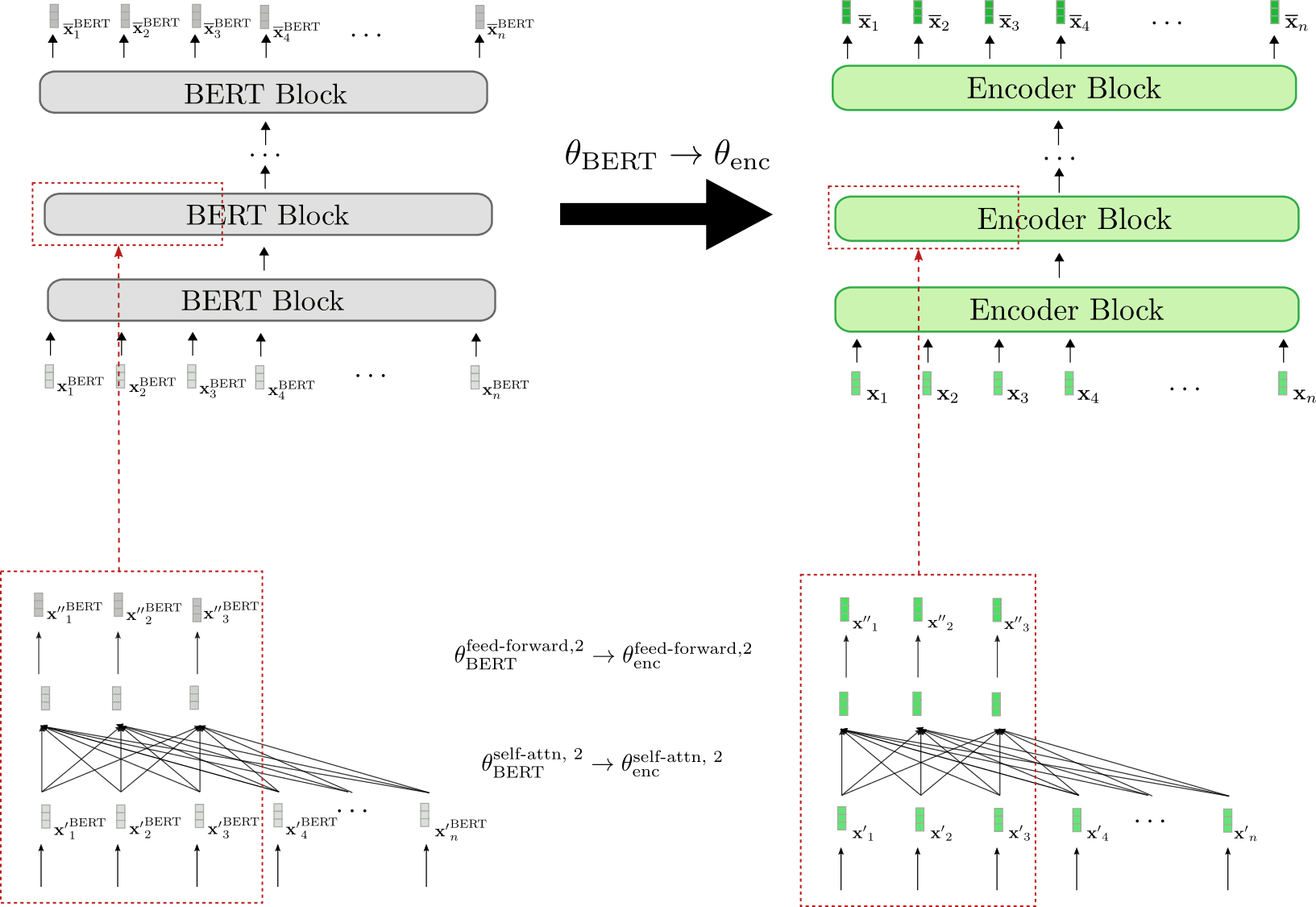
We can see that the encoder architecture corresponds 1-to-1 to BERT's architecture. The weight parameters of the bi-directional self-attention layer and the two feed-forward layers of all encoder blocks are initialized with the weight parameters of the respective BERT blocks. This is illustrated examplary for the second encoder block (red boxes at bottow) whose weight parameters θ enc self-attn , 2 \theta_{\text{enc}}^{\text{self-attn}, 2} θ enc self-attn , 2 ​ and θ enc feed-forward , 2 \theta_{\text{enc}}^{\text{feed-forward}, 2} θ enc feed-forward , 2 ​ are set to BERT's weight parameters θ BERT feed-forward , 2 \theta_{\text{BERT}}^{\text{feed-forward}, 2} θ BERT feed-forward , 2 ​ and θ BERT self-attn , 2 \theta_{\text{BERT}}^{\text{self-attn}, 2} θ BERT self-attn , 2 ​ , respectively at initialization.

Before fine-tuning, the encoder therefore behaves exactly like a pre-trained BERT model. Assuming the input sequence x 1 , … , x n \mathbf{x}_1, \ldots, \mathbf{x}_n x 1 ​ , … , x n ​ (shown in green) passed to the encoder is equal to the input sequence x 1 BERT , … , x n BERT \mathbf{x}_1^{\text{BERT}}, \ldots, \mathbf{x}_n^{\text{BERT}} x 1 BERT ​ , … , x n BERT ​ (shown in grey) passed to BERT, this means that the respective output vector sequences x ‾ 1 , … , x ‾ n \mathbf{\overline{x}}_1, \ldots, \mathbf{\overline{x}}_n x 1 ​ , … , x n ​ (shown in darker green) and x ‾ 1 BERT , … , x ‾ n BERT \mathbf{\overline{x}}_1^{\text{BERT}}, \ldots, \mathbf{\overline{x}}_n^{\text{BERT}} x 1 BERT ​ , … , x n BERT ​ (shown in darker grey) also have to be equal.

Next, let's illustrate how the decoder is warm-started.

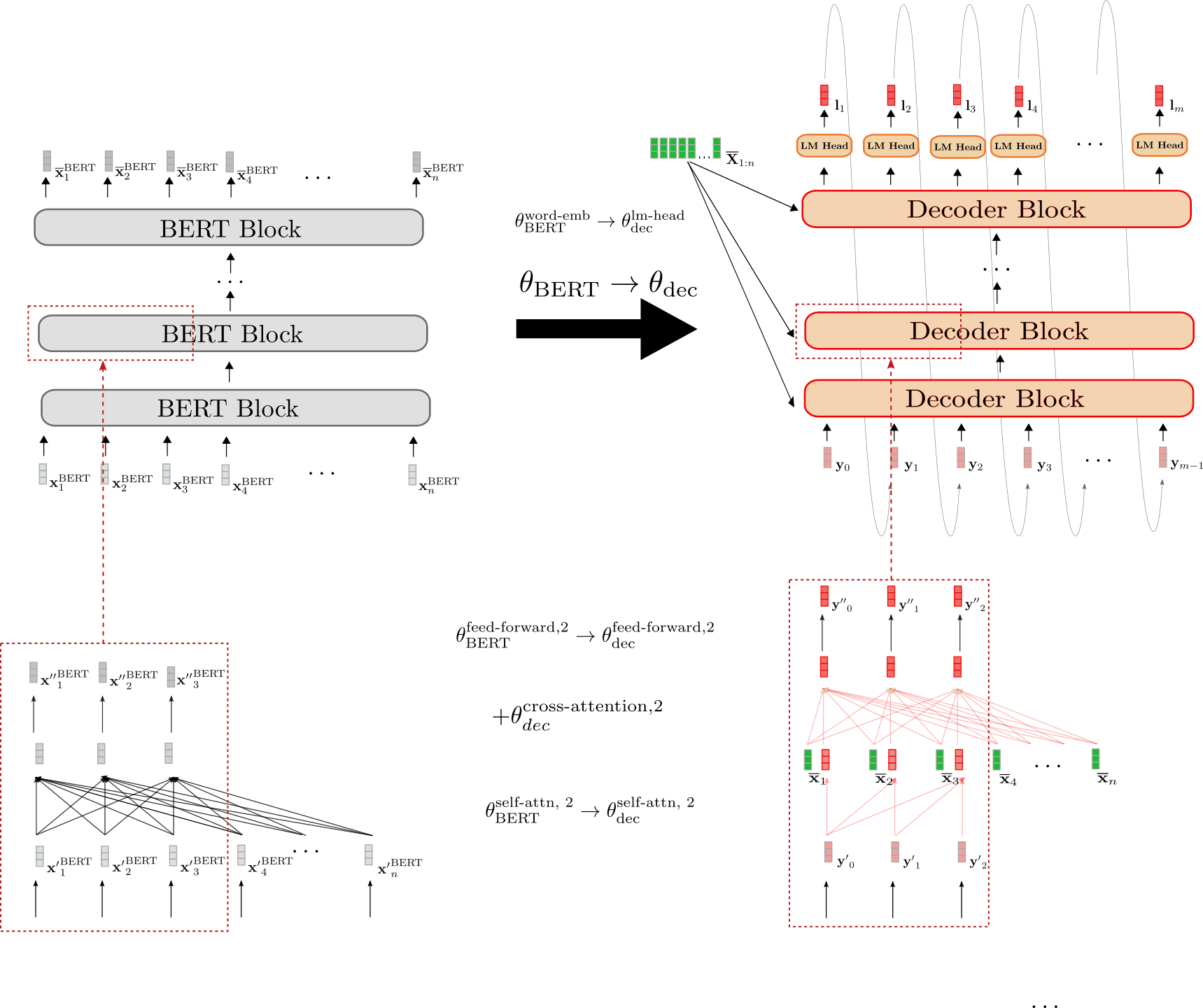
The architecture of the decoder is different from BERT's architecture in three ways.

1. First, the decoder has to be conditioned on the contextualized encoded sequence X ‾ 1 : n \mathbf{\overline{X}}_{1:n} X 1 : n ​ by means of cross-attention layers. Consequently, randomly initialized cross-attention layers are added between the self-attention layer and the two feed-forward layers in each BERT block. This is represented exemplary for the second block by + θ dec cross-attention, 2 +\theta_{\text{dec}}^{\text{cross-attention, 2}} + θ dec cross-attention, 2 ​ and illustrated by the newly added fully connected graph in red in the lower red box on the right. This necessarily changes the behavior of each modified BERT block so that an input vector, e.g. y ′ 0 \mathbf{y'}_0 y ′ 0 ​ now yields a random output vector y ′ ′ 0 \mathbf{y''}_0 y ′′ 0 ​ (highlighted by the red border around the output vector y ′ ′ 0 \mathbf{y''}_0 y ′′ 0 ​ ).
2. Second, BERT's bi-directional self-attention layers have to be changed to uni-directional self-attention layers to comply with auto-regressive generation. Because both the bi-directional and the uni-directional self-attention layer are based on the same key , query and value projection weights, the decoder's self-attention layer weights can be initialized with BERT's self-attention layer weights. E.g. the query, key and value weight parameters of the decoder's uni-directional self-attention layer are initialized with those of BERT's bi-directional self-attention layer θ BERT self-attn , 2 = { W BERT , k self-attn , 2 , W BERT , v self-attn , 2 , W BERT , q self-attn , 2 } → θ dec self-attn , 2 = { W dec , k self-attn , 2 , W dec , v self-attn , 2 , W dec , q self-attn , 2 } . \theta_{\text{BERT}}^{\text{self-attn}, 2} = \{\mathbf{W}_{\text{BERT}, k}^{\text{self-attn}, 2}, \mathbf{W}_{\text{BERT}, v}^{\text{self-attn}, 2}, \mathbf{W}_{\text{BERT}, q}^{\text{self-attn}, 2} \} \to \theta_{\text{dec}}^{\text{self-attn}, 2} = \{\mathbf{W}_{\text{dec}, k}^{\text{self-attn}, 2}, \mathbf{W}_{\text{dec}, v}^{\text{self-attn}, 2}, \mathbf{W}_{\text{dec}, q}^{\text{self-attn}, 2} \}. θ BERT self-attn , 2 ​ = { W BERT , k self-attn , 2 ​ , W BERT , v self-attn , 2 ​ , W BERT , q self-attn , 2 ​ } → θ dec self-attn , 2 ​ = { W dec , k self-attn , 2 ​ , W dec , v self-attn , 2 ​ , W dec , q self-attn , 2 ​ } . However, in uni-directional self-attention each token only attends to all previous tokens, so that the decoder's self-attention layers yield different output vectors than BERT's self-attention layers even though they share the same weights. Compare e.g. , the decoder's causally connected graph in the right box versus BERT's fully connected graph in the left box.
3. Third, the decoder outputs a sequence of logit vectors L 1 : m \mathbf{L}_{1:m} L 1 : m ​ in order to define the conditional probability distribution p θ dec ( Y 1 : n ∣ X ‾ ) p_{\theta_{\text{dec}}}(\mathbf{Y}_{1:n} | \mathbf{\overline{X}}) p θ dec ​ ​ ( Y 1 : n ​ ∣ X ) . As a result, a LM Head layer is added on top of the last decoder block. The weight parameters of the LM Head layer usually correspond to the weight parameters of the word embedding W emb \mathbf{W}_{\text{emb}} W emb ​ and thus are not randomly initialized. This is illustrated in the top by the initialization θ BERT word-emb → θ dec lm-head \theta_{\text{BERT}}^{\text{word-emb}} \to \theta_{\text{dec}}^{\text{lm-head}} θ BERT word-emb ​ → θ dec lm-head ​ .

To conclude, when warm-starting the decoder from a pre-trained BERT model only the cross-attention layer weights are randomly initialized. All other weights including those of the self-attention layer and LM Head are initialized with BERT's pre-trained weight parameters.

Having warm-stared the encoder-decoder model, the weights are then fine-tuned on a sequence-to-sequence downstream task, such as summarization.

Warm-starting Encoder-Decoder with BERT and GPT2

Instead of warm-starting both the encoder and decoder with a BERT checkpoint, we can instead leverage the BERT checkpoint for the encoder and a GPT2 checkpoint for the decoder. At first glance, a decoder-only GPT2 checkpoint seems to be better-suited to warm-start the decoder because it has already been trained on causal language modeling and uses uni-directional self-attention layers.

Let's illustrate how a GPT2 checkpoint can be used to warm-start the decoder.

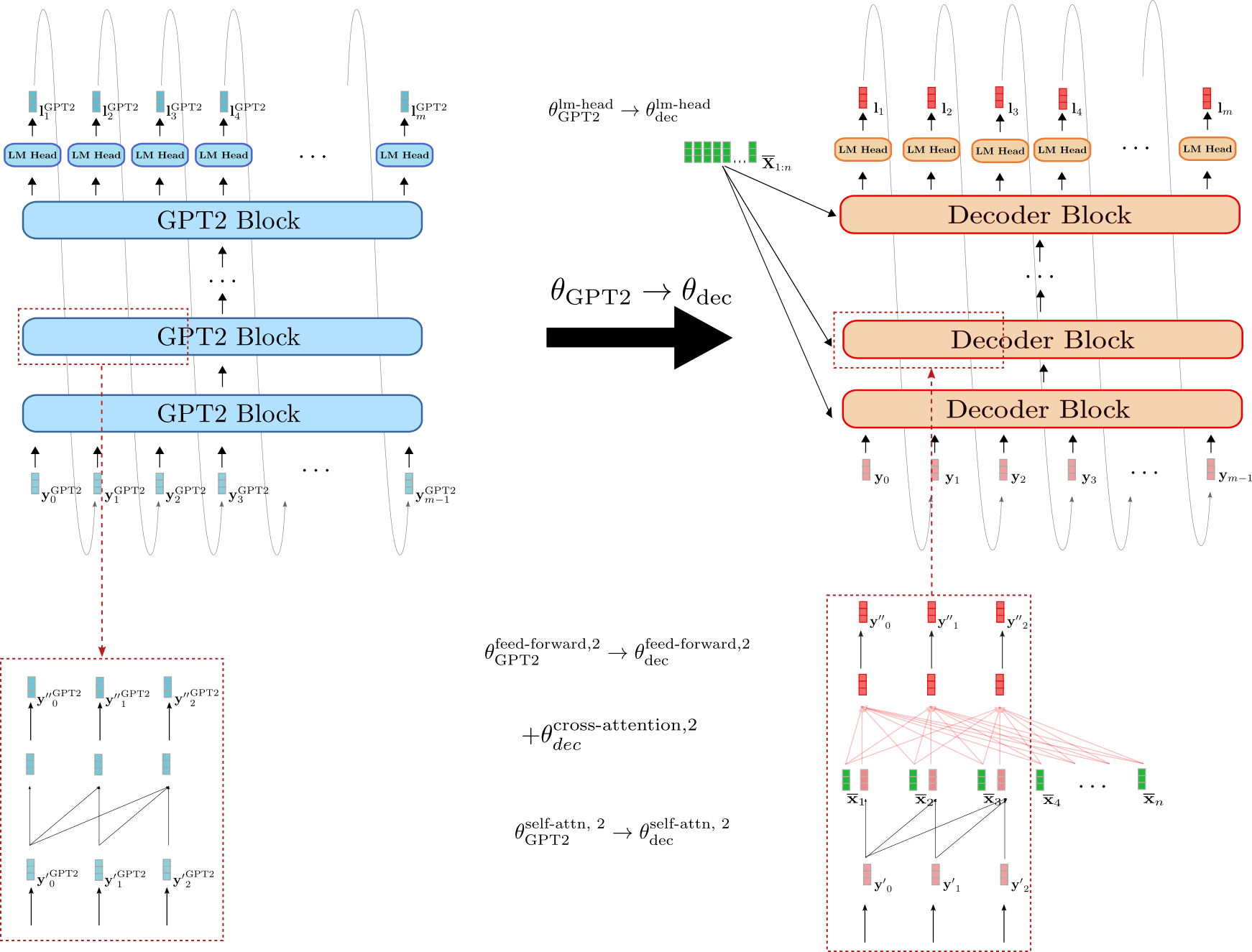
We can see that decoder is more similar to GPT2 than it is to BERT. The weight parameters of decoder's LM Head can directly be initialized with GPT2's LM Head weight parameters, e.g. θ GPT2 lm-head → θ dec lm-head \theta_{\text{GPT2}}^{\text{lm-head}} \to \theta_{\text{dec}}^{\text{lm-head}} θ GPT2 lm-head ​ → θ dec lm-head ​ . In addition, the blocks of the decoder and GPT2 both make use of uni-directional self-attention so that the output vectors of the decoder's self-attention layer are equivalent to GPT2's output vectors assuming the input vectors are the same, e.g. y ′ 0 GPT2 = y ′ 0 \mathbf{y'}_0^{\text{GPT2}} = \mathbf{y'}_0 y ′ 0 GPT2 ​ = y ′ 0 ​ . In contrast to the BERT-initialized decoder, the GPT2-initialized decoder, therefore, keeps the causal connected graph of the self-attention layer as can be seen in the red boxes on the bottom.

Nevertheless, the GPT2-initialized decoder also has to condition the decoder on X ‾ 1 : n \mathbf{\overline{X}}_{1:n} X 1 : n ​ . Analoguos to the BERT-initialized decoder, randomly initialized weight parameters for the cross-attention layer are therefore added to each decoder block. This is illustrated e.g. for the second encoder block by + θ dec cross-attention, 2 +\theta_{\text{dec}}^{\text{cross-attention, 2}} + θ dec cross-attention, 2 ​ .

Even though GPT2 resembles the decoder part of an encoder-decoder model more than BERT, a GPT2-initialized decoder will also yield random logit vectors L 1 : m \mathbf{L}_{1:m} L 1 : m ​ without fine-tuning due to randomly initialized cross-attention layers in every decoder block. It would be interesting to investigate whether a GPT2-initialized decoder yields better results or can be fine-tuned more efficiently.

Encoder-Decoder Weight Sharing

In Raffel et al. (2020) , the authors show that a randomly-initialized encoder-decoder model that shares the encoder's weights with the decoder, and therefore reduces the memory footprint by half, performs only slightly worse than its "non-shared" version. Sharing the encoder's weights with the decoder means that all layers of the decoder that are found at the same position in the encoder share the same weight parameters, i.e. the same node in the network's computation graph. E.g. the query, key, and value projection matrices of the self-attention layer in the third encoder block, defined as W Enc , k self-attn , 3 \mathbf{W}^{\text{self-attn}, 3}_{\text{Enc}, k} W Enc , k self-attn , 3 ​ , W Enc , v self-attn , 3 \mathbf{W}^{\text{self-attn}, 3}_{\text{Enc}, v} W Enc , v self-attn , 3 ​ , W Enc , q self-attn , 3 \mathbf{W}^{\text{self-attn}, 3}_{\text{Enc}, q} W Enc , q self-attn , 3 ​ are identical to the respective query, key, and value projections matrices of the self-attention layer in the third decoder block 2 {}^2 2 :

W k self-attn , 3 = W enc , k self-attn , 3 ≡ W dec , k self-attn , 3 , \mathbf{W}^{\text{self-attn}, 3}_{k} = \mathbf{W}^{\text{self-attn}, 3}_{\text{enc}, k} \equiv \mathbf{W}^{\text{self-attn}, 3}_{\text{dec}, k}, W k self-attn , 3 ​ = W enc , k self-attn , 3 ​ ≡ W dec , k self-attn , 3 ​ , W q self-attn , 3 = W enc , q self-attn , 3 ≡ W dec , q self-attn , 3 , \mathbf{W}^{\text{self-attn}, 3}_{q} = \mathbf{W}^{\text{self-attn}, 3}_{\text{enc}, q} \equiv \mathbf{W}^{\text{self-attn}, 3}_{\text{dec}, q}, W q self-attn , 3 ​ = W enc , q self-attn , 3 ​ ≡ W dec , q self-attn , 3 ​ , W v self-attn , 3 = W enc , v self-attn , 3 ≡ W dec , v self-attn , 3 , \mathbf{W}^{\text{self-attn}, 3}_{v} = \mathbf{W}^{\text{self-attn}, 3}_{\text{enc}, v} \equiv \mathbf{W}^{\text{self-attn}, 3}_{\text{dec}, v}, W v self-attn , 3 ​ = W enc , v self-attn , 3 ​ ≡ W dec , v self-attn , 3 ​ ,

As a result, the key projection weights W k self-attn , 3 , W v self-attn , 3 , W q self-attn , 3 \mathbf{W}^{\text{self-attn}, 3}_{k}, \mathbf{W}^{\text{self-attn}, 3}_{v}, \mathbf{W}^{\text{self-attn}, 3}_{q} W k self-attn , 3 ​ , W v self-attn , 3 ​ , W q self-attn , 3 ​ are updated twice for each backward propagation pass - once when the gradient is backpropagated through the third decoder block and once when the gradient is backprapageted thourgh the third encoder block.

In the same way, we can warm-start an encoder-decoder model by sharing the encoder weights with the decoder. Being able to share the weights between the encoder and decoder requires the decoder architecture (excluding the cross-attention weights) to be identical to the encoder architecture. Therefore, encoder-decoder weight sharing is only relevant if the encoder-decoder model is warm-started from a single encoder-only pre-trained checkpoint.

Great! That was the theory about warm-starting encoder-decoder models. Let's now look at some results.

1 {}^1 1 Without loss of generality, we exclude the normalization layers to not clutter the equations and illustrations. 2 {}^2 2 For more detail on how self-attention layers function, please refer to this section of the transformer-based encoder-decoder model blog post for the encoder-part (and this section for the decoder part respectively).

Warm-starting encoder-decoder models (Analysis)

In this section, we will summarize the findings on warm-starting encoder-decoder models as presented in Leveraging Pre-trained Checkpoints for Sequence Generation Tasks by Sascha Rothe, Shashi Narayan, and Aliaksei Severyn. The authors compared the performance of warm-started encoder-decoder models to randomly initialized encoder-decoder models on multiple sequence-to-sequence tasks, notably summarization , translation , sentence splitting , and sentence fusion .

To be more precise, the publicly available pre-trained checkpoints of BERT , RoBERTa , and GPT2 were leveraged in different variations to warm-start an encoder-decoder model. E.g. a BERT-initialised encoder was paired with a BERT-initialized decoder yielding a BERT2BERT model or a RoBERTa-initialized encoder was paired with a GPT2-initialized decoder to yield a RoBERTa2GPT2 model. Additionally, the effect of sharing the encoder and decoder weights (as explained in the previous section) was investigated for RoBERTa, i.e. RoBERTaShare , and for BERT, i.e. BERTShare . Randomly or partly randomly initialized encoder-decoder models were used as a baseline, such as a fully randomly initialized encoder-decoder model, coined Rnd2Rnd or a BERT-initialized decoder paired with a randomly initialized encoder, defined as Rnd2BERT .

The following table shows a complete list of all investigated model variants including the number of randomly initialized weights, i.e. "random", and the number of weights initialized from the respective pre-trained checkpoints, i.e. "leveraged". All models are based on a 12-layer architecture with 768-dim hidden size embeddings, corresponding to the bert-base-cased , bert-base-uncased , roberta-base , and gpt2 checkpoints in the 🤗Transformers model hub.

The model Rnd2Rnd , which is based on the BERT2BERT architecture, contains 221M weight parameters - all of which are randomly initialized. The other two "BERT-based" baselines Rnd2BERT and BERT2Rnd have roughly half of their weights, i.e. 112M parameters, randomly initialized. The other 109M weight parameters are leveraged from the pre-trained bert-base-uncased checkpoint for the encoder- or decoder part respectively. The models BERT2BERT , BERT2GPT2 , and RoBERTa2GPT2 have all of their encoder weight parameters leveraged (from bert-base-uncased , roberta-base respectively) and most of the decoder weight parameter weights as well (from gpt2 , bert-base-uncased respectively). 26M decoder weight parameters, which correspond to the 12 cross-attention layers, are thereby randomly initialized. RoBERTa2GPT2 and BERT2GPT2 are compared to the Rnd2GPT2 baseline. Also, it should be noted that the shared model variants BERTShare and RoBERTaShare have significantly fewer parameters because all encoder weight parameters are shared with the respective decoder weight parameters.

Experiments

The above models were trained and evaluated on four sequence-to-sequence tasks of increasing complexity: sentence-level fusion, sentence-level splitting, translation, and abstractive summarization. The following table shows which datasets were used for each task.

Depending on the task, a slightly different training regime was used. E.g. according to the size of the dataset and the specific task, the number of training steps ranges from 200K to 500K, the batch size is set to either 128 or 256, the input length ranges from 128 to 512 and the output length varies between 32 to 128. It shall be emphasized however that within each task, all models were trained and evaluated using the same hyperparameters to ensure a fair comparison. For more information on the task-specific hyperparameter settings, the reader is advised to see the Experiments section in the paper .

We will now give a condensed overview of the results for each task.

Sentence Fusion and -Splitting (DiscoFuse, WikiSplit)

Sentence Fusion is the task of combining multiple sentences into a single coherent sentence. E.g. the two sentences:

As a run-blocker, Zeitler moves relatively well. Zeitler too often struggles at the point of contact in space.

should be connected with a fitting linking word , such as:

As a run-blocker, Zeitler moves relatively well. However , he too often struggles at the point of contact in space.

As can be seen the linking word "however" provides a coherent transition from the first sentence to the second one. A model that is capable of generating such a linking word has arguably learned to infer that the two sentences above contrast to each other.

The inverse task is called Sentence splitting and consists of splitting a single complex sentence into multiple simpler ones that together retain the same meaning. Sentence splitting is considered as an important task in text simplification, cf. to Botha et al. (2018) .

As an example, the sentence:

Street Rod is the first in a series of two games released for the PC and Commodore 64 in 1989

can be simplified into

Street Rod is the first in a series of two games . It was released for the PC and Commodore 64 in 1989

It can be seen that the long sentence tries to convey two important pieces of information. One is that the game was the first of two games being released for the PC, and the second being the year in which it was released. Sentence splitting, therefore, requires the model to understand which part of the sentence should be divided into two sentences, making the task more difficult than sentence fusion.

A common metric to evaluate the performance of models on sentence fusion resp. -splitting tasks is SARI (Wu et al. (2016) , which is broadly based on the F1-score of label and model output.

Let's see how the models perform on sentence fusion and -splitting.

The first two columns show the performance of the encoder-decoder models on the DiscoFuse evaluation data. The first column states the results of encoder-decoder models trained on all (100%) of the training data, while the second column shows the results of the models trained only on 10% of the training data. We observe that warm-started models perform significantly better than the randomly initialized baseline models Rnd2Rnd , Rnd2Bert , and Rnd2GPT2 . A warm-started RoBERTa2GPT2 model trained only on 10% of the training data is on par with an Rnd2Rnd model trained on 100% of the training data. Interestingly, the Bert2Rnd baseline performs equally well as a fully warm-started Bert2Bert model, which indicates that warm-starting the encoder-part is more effective than warm-starting the decoder-part. The best results are obtained by RoBERTa2GPT2 , followed by RobertaShare . Sharing encoder and decoder weight parameters does seem to slightly increase the model's performance.

On the more difficult sentence splitting task, a similar pattern emerges. Warm-started encoder-decoder models significantly outperform encoder-decoder models whose encoder is randomly initialized and encoder-decoder models with shared weight parameters yield better results than those with uncoupled weight parameters. On sentence splitting the BertShare models yields the best performance closely followed by RobertaShare .

In addition to the 12-layer model variants, the authors also trained and evaluated a 24-layer RobertaShare (large) model which outperforms all 12-layer models significantly.

Machine Translation (WMT14)

Next, the authors evaluated warm-started encoder-decoder models on the probably most common benchmark in machine translation (MT) - the En → \to → De and De → \to → En WMT14 dataset. In this notebook, we present the results on the newstest2014 eval dataset. Because the benchmark requires the model to understand both an English and a German vocabulary the BERT-initialized encoder-decoder models were warm-started from the multilingual pre-trained checkpoint bert-base-multilingual-cased . Because there is no publicly available multilingual RoBERTa checkpoint, RoBERTa-initialized encoder-decoder models were excluded for MT. GPT2-initialized models were initialized from the gpt2 pre-trained checkpoint as in the previous experiment. The translation results are reported using the BLUE-4 score metric 1 {}^1 1 .

Again, we observe a significant performance boost by warm-starting the encoder-part, with BERT2Rnd and BERT2BERT yielding the best results on both the En → \to → De and De → \to → En tasks. GPT2 initialized models perform significantly worse even than the Rnd2Rnd baseline on En → \to → De . Taking into consideration that the gpt2 checkpoint was trained only on English text, it is not very surprising that BERT2GPT2 and Rnd2GPT2 models have difficulties generating German translations. This hypothesis is supported by the competitive results ( e.g. 31.4 vs. 32.7) of BERT2GPT2 on the De → \to → En task for which GPT2's vocabulary fits the English output format. Contrary to the results obtained on sentence fusion and sentence splitting, sharing encoder and decoder weight parameters does not yield a performance boost in MT. Possible reasons for this as stated by the authors include

• the encoder-decoder model capacity is an important factor in MT, and
• the encoder and decoder have to deal with different grammar and vocabulary

Since the bert-base-multilingual-cased checkpoint was trained on more than 100 languages, its vocabulary is probably undesirably large for En → \to → De and De → \to → En MT. Thus, the authors pre-trained a large BERT encoder-only checkpoint on the English and German subset of the Wikipedia dump and subsequently used it to warm-start a BERT2Rnd and BERTShare encoder-decoder model. Thanks to the improved vocabulary, another significant performance boost is observed, with BERT2Rnd (large, custom) significantly outperforming all other models.

Summarization (CNN/Dailymail, BBC XSum, Gigaword)

Finally, the encoder-decoder models were evaluated on the arguably most challenging sequence-to-sequence task - summarization . The authors picked three summarization datasets with different characteristics for evaluation: Gigaword ( headline generation ), BBC XSum ( extreme summarization ), and CNN/Dailymayl ( abstractive summarization ).

The Gigaword dataset contains sentence-level abstractive summarizations, requiring the model to learn sentence-level understanding, abstraction, and eventually paraphrasing. A typical data sample in Gigaword, such as

"*venezuelan president hugo chavez said thursday he has ordered a probe into a suspected coup plot allegedly involving active and retired military officers .*",

would have a corresponding headline as its label, e.g. :

" chavez orders probe into suspected coup plot ".

The BBC XSum dataset consists of much longer article-like text inputs with the labels being mostly single sentence summarizations. This dataset requires the model not only to learn document-level inference but also a high level of abstractive paraphrasing. Some data samples of the BBC XSUM datasets are shown here .

For the CNN/Dailmail dataset, documents, which are of similar length than those in the BBC XSum dataset, have to be summarized to bullet-point story highlights. The labels therefore often consist of multiple sentences. Besides document-level understanding, the CNN/Dailymail dataset requires models to be good at copying the most salient information. Some examples can be viewed here .

The models are evaluated using the Rouge metric , whereas the Rouge-2 scores are shown below.

Alright, let's take a look at the results.

We observe again that warm-starting the encoder-part gives a significant improvement over models with randomly-initialized encoders, which is especially visible for document-level abstraction tasks, i.e. CNN/Dailymail and BBC XSum. This shows that tasks requiring a high level of abstraction benefit more from a pre-trained encoder part than those requiring only sentence-level abstraction. Except for Gigaword GPT2-based encoder-decoder models seem to be unfit for summarization.