Fine-tuning LLMs to 1.58bit: extreme quantization made easy

Fine-tuning LLMs to 1.58bit: extreme quantization made easy

• +274

As Large Language Models (LLMs) grow in size and complexity, finding ways to reduce their computational and energy costs has become a critical challenge. One popular solution is quantization, where the precision of parameters is reduced from the standard 16-bit floating-point (FP16) or 32-bit floating-point (FP32) to lower-bit formats like 8-bit or 4-bit. While this approach significantly cuts down on memory usage and speeds up computation, it often comes at the expense of accuracy. Reducing the precision too much can cause models to lose crucial information, resulting in degraded performance.

BitNet is a special transformers architecture that represents each parameter with only three values: (-1, 0, 1) , offering a extreme quantization of just 1.58 ( l o g 2 ( 3 ) log_2(3) l o g 2 ​ ( 3 ) ) bits per parameter. However, it requires to train a model from scratch. While the results are impressive, not everybody has the budget to pre-train an LLM. To overcome this limitation, we explored a few tricks that allow fine-tuning an existing model to 1.58 bits! Keep reading to find out how !

Table of Contents

• TL;DR
• What is BitNet in More Depth?
• Pre-training Results in 1.58b
• Fine-tuning in 1.58b
• Kernels used & Benchmarks
• Conclusion
• Acknowledgements
• Additional Resources

TL;DR

BitNet is an architecture introduced by Microsoft Research that uses extreme quantization, representing each parameter with only three values: -1, 0, and 1. This results in a model that uses just 1.58 bits per parameter, significantly reducing computational and memory requirements.

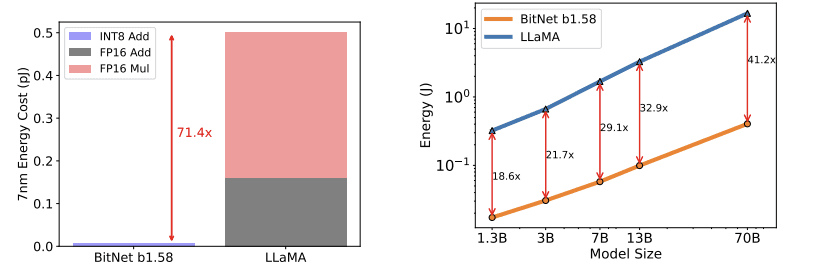
This architecture uses INT8 addition calculations when performing matrix multiplication, in contrast to LLaMA LLM's FP16 addition and multiplication operations.

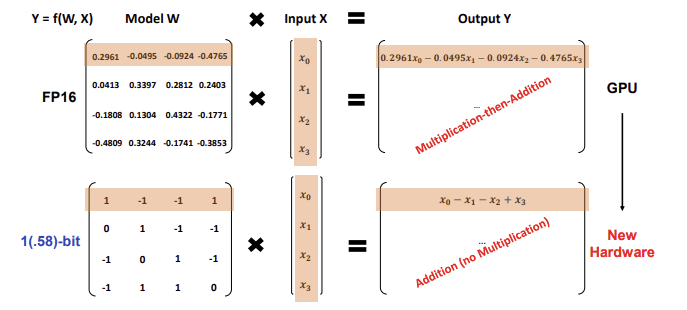
This results in a theoretically reduced energy consumption, with BitNet b1.58 saving 71.4 times the arithmetic operations energy for matrix multiplication compared to the Llama baseline.

We have successfully fine-tuned a Llama3 8B model using the BitNet architecture, achieving strong performance on downstream tasks. The 8B models we developed are released under the HF1BitLLM organization. Two of these models were fine-tuned on 10B tokens with different training setup, while the third was fine-tuned on 100B tokens. Notably, our models surpass the Llama 1 7B model in MMLU benchmarks.

How to Use with Transformers

To integrate the BitNet architecture into Transformers, we introduced a new quantization method called "bitnet" ( PR ). This method involves replacing the standard Linear layers with specialized BitLinear layers that are compatible with the BitNet architecture, with appropriate dynamic quantization of activations, weight unpacking, and matrix multiplication.

Loading and testing the model in Transformers is incredibly straightforward, there are zero changes to the API:

model = AutoModelForCausalLM.from_pretrained(
    "HF1BitLLM/Llama3-8B-1.58-100B-tokens",
    device_map="cuda",
    torch_dtype=torch.bfloat16
)    
tokenizer = AutoTokenizer.from_pretrained("meta-llama/Meta-Llama-3-8B-Instruct")

input_text = "Daniel went back to the garden. Mary travelled to the kitchen. Sandra journeyed to the kitchen. Sandra went to the hallway. John went to the bedroom. Mary went back to the garden. Where is Mary?\nAnswer:"

input_ids = tokenizer.encode(input_text, return_tensors="pt").cuda()
output = model.generate(input_ids, max_new_tokens=10)
generated_text = tokenizer.decode(output[0], skip_special_tokens=True)
print(generated_text)

With this code, everything is managed seamlessly behind the scenes, so there's no need to worry about additional complexities, you just need to install the latest version of transformers.

For a quick test of the model, check out this notebook

What is BitNet In More Depth?

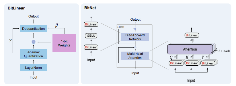
BitNet replaces traditional Linear layers in Multi-Head Attention and Feed-Forward Networks with specialized layers called BitLinear that use ternary precision (or even binary, in the initial version). The BitLinear layers we use in this project quantize the weights using ternary precision (with values of -1, 0, and 1), and we quantize the activations to 8-bit precision. We use a different implementation of BitLinear for training than we do for inference, as we'll see in the next section.

The main obstacle to training in ternary precision is that the weight values are discretized (via the round() function) and thus non-differentiable. BitLinear solves this with a nice trick: STE (Straight Through Estimator) . The STE allows gradients to flow through the non-differentiable rounding operation by approximating its gradient as 1 (treating round() as equivalent to the identity function). Another way to view it is that, instead of stopping the gradient at the rounding step, the STE lets the gradient pass through as if the rounding never occurred, enabling weight updates using standard gradient-based optimization techniques.

Training

We train in full precision, but quantize the weights into ternary values as we go, using symmetric per tensor quantization. First, we compute the average of the absolute values of the weight matrix and use this as a scale. We then divide the weights by the scale, round the values, constrain them between -1 and 1, and finally rescale them to continue in full precision.

s c a l e w = 1 1 n m ∑ i j ∣ W i j ∣ scale_w = \frac{1}{\frac{1}{nm} \sum_{ij} |W_{ij}|} sc a l e w ​ = nm 1 ​ ∑ ij ​ ∣ W ij ​ ∣ 1 ​

W q = clamp [ − 1 , 1 ] ( round ( W ∗ s c a l e ) ) W_q = \text{clamp}_{[-1,1]}(\text{round}(W*scale)) W q ​ = clamp [ − 1 , 1 ] ​ ( round ( W ∗ sc a l e ))

W d e q u a n t i z e d = W q ∗ s c a l e w W_{dequantized} = W_q*scale_w W d e q u an t i ze d ​ = W q ​ ∗ sc a l e w ​

Activations are then quantized to a specified bit-width (8-bit, in our case) using absmax per token quantization (for a comprehensive introduction to quantization methods check out this post ). This involves scaling the activations into the range [−128, 127] for an 8-bit bit-width. The quantization formula is:

s c a l e x = 127 ∣ X ∣ max ,   dim = − 1 scale_x = \frac{127}{|X|_{\text{max}, \, \text{dim}=-1}} sc a l e x ​ = ∣ X ∣ max , dim = − 1 ​ 127 ​

X q = clamp [ − 128 , 127 ] ( round ( X ∗ s c a l e ) ) X_q = \text{clamp}_{[-128,127]}(\text{round}(X*scale)) X q ​ = clamp [ − 128 , 127 ] ​ ( round ( X ∗ sc a l e ))

X d e q u a n t i z e d = X q ∗ s c a l e x X_{dequantized} = X_q * scale_x X d e q u an t i ze d ​ = X q ​ ∗ sc a l e x ​

To make the formulas clearer, here are examples of weight and activation quantization using a 3x3 matrix:

Let the weight matrix ( W ) be:

W = [ 0.8 − 0.5 1.2 − 1.5 0.4 − 0.9 1.3 − 0.7 0.2 ] W = \begin{bmatrix} 0.8 & -0.5 & 1.2 \\ -1.5 & 0.4 & -0.9 \\ 1.3 & -0.7 & 0.2 \end{bmatrix} W = ​ 0.8 − 1.5 1.3 ​ − 0.5 0.4 − 0.7 ​ 1.2 − 0.9 0.2 ​ ​

Step 1: Compute the Scale for Weights

Using the formula:

s c a l e w = 1 1 n m ∑ i j ∣ W i j ∣ scale_w = \frac{1}{\frac{1}{nm} \sum_{ij} |W_{ij}|} sc a l e w ​ = nm 1 ​ ∑ ij ​ ∣ W ij ​ ∣ 1 ​

we calculate the average absolute value of ( W ):

1 n m ∑ i j ∣ W i j ∣ = 1 9 ( 0.8 + 0.5 + 1.2 + 1.5 + 0.4 + 0.9 + 1.3 + 0.7 + 0.2 ) = 1 9 ( 7.5 ) = 0.8333 \frac{1}{nm} \sum_{ij} |W_{ij}| = \frac{1}{9}(0.8 + 0.5 + 1.2 + 1.5 + 0.4 + 0.9 + 1.3 + 0.7 + 0.2) = \frac{1}{9}(7.5) = 0.8333 nm 1 ​ ∑ ij ​ ∣ W ij ​ ∣ = 9 1 ​ ( 0.8 + 0.5 + 1.2 + 1.5 + 0.4 + 0.9 + 1.3 + 0.7 + 0.2 ) = 9 1 ​ ( 7.5 ) = 0.8333

Now, the scale factor is:

s c a l e w = 1 0.8333 ≈ 1.2 scale_w = \frac{1}{0.8333} \approx 1.2 sc a l e w ​ = 0.8333 1 ​ ≈ 1.2

Step 2: Quantize the Weight Matrix

Using the formula:

W q = clamp [ − 1 , 1 ] ( round ( W × s c a l e w ) ) W_q = \text{clamp}_{[-1, 1]}(\text{round}(W \times scale_w)) W q ​ = clamp [ − 1 , 1 ] ​ ( round ( W × sc a l e w ​ ))

We first scale the weights by s c a l e w ≈ 1.2 scale_w \approx 1.2 sc a l e w ​ ≈ 1.2 :

W × s c a l e w = [ 0.8 × 1.2 − 0.5 × 1.2 1.2 × 1.2 − 1.5 × 1.2 0.4 × 1.2 − 0.9 × 1.2 1.3 × 1.2 − 0.7 × 1.2 0.2 × 1.2 ] = [ 0.96 − 0.6 1.44 − 1.8 0.48 − 1.08 1.56 − 0.84 0.24 ] W \times scale_w = \begin{bmatrix} 0.8 \times 1.2 & -0.5 \times 1.2 & 1.2 \times 1.2 \\ -1.5 \times 1.2 & 0.4 \times 1.2 & -0.9 \times 1.2 \\ 1.3 \times 1.2 & -0.7 \times 1.2 & 0.2 \times 1.2 \end{bmatrix} = \begin{bmatrix} 0.96 & -0.6 & 1.44 \\ -1.8 & 0.48 & -1.08 \\ 1.56 & -0.84 & 0.24 \end{bmatrix} W × sc a l e w ​ = ​ 0.8 × 1.2 − 1.5 × 1.2 1.3 × 1.2 ​ − 0.5 × 1.2 0.4 × 1.2 − 0.7 × 1.2 ​ 1.2 × 1.2 − 0.9 × 1.2 0.2 × 1.2 ​ ​ = ​ 0.96 − 1.8 1.56 ​ − 0.6 0.48 − 0.84 ​ 1.44 − 1.08 0.24 ​ ​

Next, we round the values and clamp them to the range [ − 1 , 1 ] [-1, 1] [ − 1 , 1 ] :

W q = [ 1 − 1 1 − 1 0 − 1 1 − 1 0 ] W_q = \begin{bmatrix} 1 & -1 & 1 \\ -1 & 0 & -1 \\ 1 & -1 & 0 \end{bmatrix} W q ​ = ​ 1 − 1 1 ​ − 1 0 − 1 ​ 1 − 1 0 ​ ​

Step 3: Dequantize the Weights

Finally, we dequantize the weights using:

W d e q u a n t i z e d = W q × s c a l e w W_{dequantized} = W_q \times scale_w W d e q u an t i ze d ​ = W q ​ × sc a l e w ​

Substituting scale_w, we get:

W d e q u a n t i z e d = [ 1 × 1.2 − 1 × 1.2 1 × 1.2 − 1 × 1.2 0 × 1.2 − 1 × 1.2 1 × 1.2 − 1 × 1.2 0 × 1.2 ] = [ 1.2 − 1.2 1.2 − 1.2 0 − 1.2 1.2 − 1.2 0 ] W_{dequantized} = \begin{bmatrix} 1 \times 1.2 & -1 \times 1.2 & 1 \times 1.2 \\ -1 \times 1.2 & 0 \times 1.2 & -1 \times 1.2 \\ 1 \times 1.2 & -1 \times 1.2 & 0 \times 1.2 \end{bmatrix} = \begin{bmatrix} 1.2 & -1.2 & 1.2 \\ -1.2 & 0 & -1.2 \\ 1.2 & -1.2 & 0 \end{bmatrix} W d e q u an t i ze d ​ = ​ 1 × 1.2 − 1 × 1.2 1 × 1.2 ​ − 1 × 1.2 0 × 1.2 − 1 × 1.2 ​ 1 × 1.2 − 1 × 1.2 0 × 1.2 ​ ​ = ​ 1.2 − 1.2 1.2 ​ − 1.2 0 − 1.2 ​ 1.2 − 1.2 0 ​ ​

Let the activation matrix ( X ) be:

X = [ 1.0 − 0.6 0.7 − 0.9 0.4 − 1.2 0.8 − 0.5 0.3 ] X = \begin{bmatrix} 1.0 & -0.6 & 0.7 \\ -0.9 & 0.4 & -1.2 \\ 0.8 & -0.5 & 0.3 \end{bmatrix} X = ​ 1.0 − 0.9 0.8 ​ − 0.6 0.4 − 0.5 ​ 0.7 − 1.2 0.3 ​ ​

Step 1: Compute the Scale for Activations

For each row (or channel), compute the maximum absolute value:

• Row 1 : Maximum absolute value = 1.0
• Row 2 : Maximum absolute value = 1.2
• Row 3 : Maximum absolute value = 0.8

Compute the scale factors for each row:

scale = [ 127 1.0 127 1.2 127 0.8 ] = [ 127 105.83 158.75 ] \text{scale} = \begin{bmatrix} \frac{127}{1.0} \\ \frac{127}{1.2} \\ \frac{127}{0.8} \end{bmatrix} = \begin{bmatrix} 127 \\ 105.83 \\ 158.75 \end{bmatrix} scale = ​ 1.0 127 ​ 1.2 127 ​ 0.8 127 ​ ​ ​ = ​ 127 105.83 158.75 ​ ​

Step 2: Quantize the Activation Matrix

Using the formula:

X q = clamp [ − 128 , 127 ] ( round ( X × scale ) ) X_q = \text{clamp}_{[-128,127]}(\text{round}(X \times \text{scale})) X q ​ = clamp [ − 128 , 127 ] ​ ( round ( X × scale ))

Scale the activations:

X × scale = [ 1.0 × 127 − 0.6 × 127 0.7 × 127 − 0.9 × 105.83 0.4 × 105.83 − 1.2 × 105.83 0.8 × 158.75 − 0.5 × 158.75 0.3 × 158.75 ] = [ 127 − 76.2 88.9 − 95.2 42.3 − 127 127 − 79.4 47.6 ] X \times \text{scale} = \begin{bmatrix} 1.0 \times 127 & -0.6 \times 127 & 0.7 \times 127 \\ -0.9 \times 105.83 & 0.4 \times 105.83 & -1.2 \times 105.83 \\ 0.8 \times 158.75 & -0.5 \times 158.75 & 0.3 \times 158.75 \end{bmatrix} = \begin{bmatrix} 127 & -76.2 & 88.9 \\ -95.2 & 42.3 & -127 \\ 127 & -79.4 & 47.6 \end{bmatrix} X × scale = ​ 1.0 × 127 − 0.9 × 105.83 0.8 × 158.75 ​ − 0.6 × 127 0.4 × 105.83 − 0.5 × 158.75 ​ 0.7 × 127 − 1.2 × 105.83 0.3 × 158.75 ​ ​ = ​ 127 − 95.2 127 ​ − 76.2 42.3 − 79.4 ​ 88.9 − 127 47.6 ​ ​

Round the values and clamp them to the range [ − 128 , 127 ] [-128, 127] [ − 128 , 127 ] :

X q = [ 127 − 76 89 − 95 42 − 127 127 − 79 48 ] X_q = \begin{bmatrix} 127 & -76 & 89 \\ -95 & 42 & -127 \\ 127 & -79 & 48 \end{bmatrix} X q ​ = ​ 127 − 95 127 ​ − 76 42 − 79 ​ 89 − 127 48 ​ ​

Step 3: Dequantize the Activations

Finally, dequantize the activations using:

X d e q u a n t i z e d = X q × 1 scale X_{dequantized} = X_q \times \frac{1}{\text{scale}} X d e q u an t i ze d ​ = X q ​ × scale 1 ​

Substituting the scales:

X d e q u a n t i z e d = [ 127 × 1 127 − 76 × 1 127 89 × 1 127 − 95 × 1 105.83 42 × 1 105.83 − 127 × 1 105.83 127 × 1 158.75 − 79 × 1 158.75 48 × 1 158.75 ] = [ 1.0 − 0.6 0.7 − 0.9 0.4 − 1.2 0.8 − 0.5 0.3 ] X_{dequantized} = \begin{bmatrix} 127 \times \frac{1}{127} & -76 \times \frac{1}{127} & 89 \times \frac{1}{127} \\ -95 \times \frac{1}{105.83} & 42 \times \frac{1}{105.83} & -127 \times \frac{1}{105.83} \\ 127 \times \frac{1}{158.75} & -79 \times \frac{1}{158.75} & 48 \times \frac{1}{158.75} \end{bmatrix} = \begin{bmatrix} 1.0 & -0.6 & 0.7 \\ -0.9 & 0.4 & -1.2 \\ 0.8 & -0.5 & 0.3 \end{bmatrix} X d e q u an t i ze d ​ = ​ 127 × 127 1 ​ − 95 × 105.83 1 ​ 127 × 158.75 1 ​ ​ − 76 × 127 1 ​ 42 × 105.83 1 ​ − 79 × 158.75 1 ​ ​ 89 × 127 1 ​ − 127 × 105.83 1 ​ 48 × 158.75 1 ​ ​ ​ = ​ 1.0 − 0.9 0.8 ​ − 0.6 0.4 − 0.5 ​ 0.7 − 1.2 0.3 ​ ​

We apply Layer Normalization (LN) before quantizing the activations to maintain the variance of the output:

LN ( x ) = x − E ( x ) Var ( x ) + ϵ \text{LN}(x) = \frac{x - E(x)}{\sqrt{\text{Var}(x) + \epsilon}} LN ( x ) = Var ( x ) + ϵ ​ x − E ( x ) ​

where ϵ is a small number to prevent overflow.

The round() function is not differentiable, as mentioned before. We use detach() as a trick to implement a differentiable straight-through estimator in the backward pass:

# Adapted from https://github.com/microsoft/unilm/blob/master/bitnet/The-Era-of-1-bit-LLMs__Training_Tips_Code_FAQ.pdf
import torch
import torch.nn as nn 
import torch.nn.functional as F

def activation_quant(x):
    scale = 127.0 / x.abs().max(dim=-1, keepdim=True).values.clamp_(min=1e-5)
    y = (x * scale).round().clamp_(-128, 127) / scale
    return y
 
def weight_quant(w):
    scale = 1.0 / w.abs().mean().clamp_(min=1e-5)
    u = (w * scale).round().clamp_(-1, 1) / scale
    return u

class BitLinear(nn.Linear):
    """
    Only for training
    """
    def forward(self, x):
        w = self.weight
        x_norm = LN(x)
        
        # A trick for implementing Straight−Through−Estimator (STE) using detach()
        x_quant = x_norm + (activation_quant(x_norm) - x_norm).detach()
        w_quant = w + (weight_quant(w) - w).detach()
        
        # Perform quantized linear transformation
        y = F.linear(x_quant, w_quant)
        return y

Inference

During inference, we simply quantize the weights to ternary values without rescaling. We apply the same approach to activations using 8-bit precision, then perform a matrix multiplication with an efficient kernel, followed by dividing by both the weight and activation scales. This should significantly improve inference speed, particularly with optimized hardware. You can see that the rescaling process differs during training, as matrix multiplications are kept in fp16/bf16/fp32 for proper training.

# Adapted from https://github.com/microsoft/unilm/blob/master/bitnet/The-Era-of-1-bit-LLMs__Training_Tips_Code_FAQ.pdf
import torch
import torch.nn as nn 
import torch.nn.functional as F

def activation_quant_inference(x):
    x = LN(x)
    scale = 127.0 / x.abs().max(dim=-1, keepdim=True).values.clamp_(min=1e-5)
    y = (x * scale).round().clamp_(-128, 127)
    return y, scale
 
class BitLinear(nn.Linear):
    """
    Only for training
    """
    def forward(self, x):
        w = self.weight # weights here are already quantized to (-1, 0, 1)    
        w_scale = self.w_scale  
        x_quant, x_scale = activation_quant_inference(x)
        y = efficient_kernel(x_quant, w) / w_scale / x_scale
        return y

Pre-training Results in 1.58b

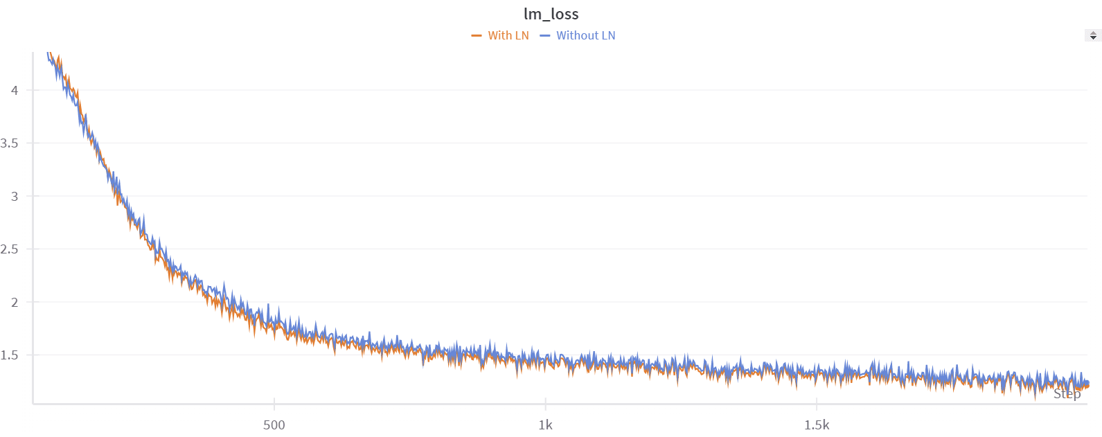
Before attempting fine-tuning, we first tried to reproduce the results of the BitNet paper with pre-training. We started with a small dataset, tinystories , and a Llama3 8B model . We confirmed that adding a normalization function, like the paper does, improves performance. For example, after 2000 steps of training, we had a perplexity on the validation set equal to 6.3 without normalization, and 5.9 with normalization. Training was stable in both cases.

While this approach looks very interesting for pre-training, only a few institutions can afford doing it at the necessary scale. However, there is already a wide range of strong pretrained models, and it would be extremely useful if they could be converted to 1.58bit after pre-training. Other groups had reported that fine-tuning results were not as strong as those achieved with pre-training, so we set out on an investigation to see if we could make 1.58 fine-tuning work.

Fine-tuning in 1.58bit

When we began fine-tuning from the pre-trained Llama3 8B weights, the model performed slightly better but not as well as we expected.

Note: All our experiments were conducted using Nanotron . If you're interested in trying 1.58bit pre-training or fine-tuning, you can check out this PR .

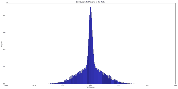
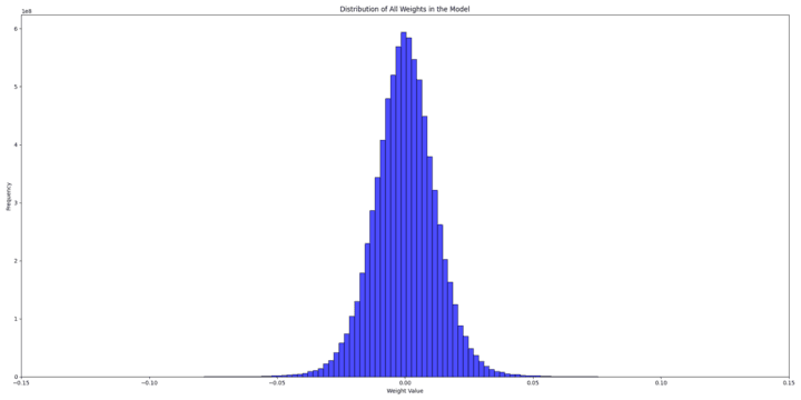
To understand why, we tried to inspect both the weight distributions of the randomly initialized model and the pre-trained model to identify potential issues.

And the scale values for the two distributions are, respectively :

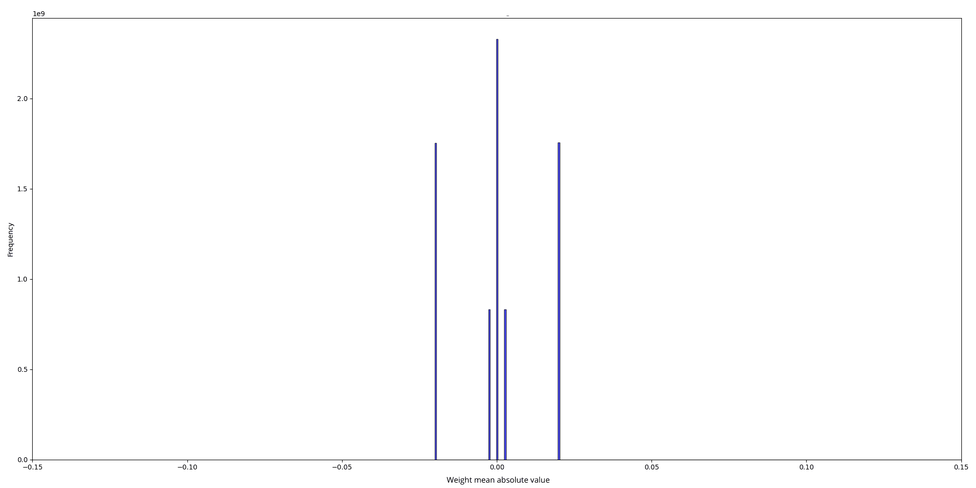
The initial random weight distribution is a mix of two normal distributions:

• One with a standard deviation (std) of 0.025 0.025 0.025
• Another with a std of 0.025 2 ⋅ num_hidden_layers = 0.00325 \frac{0.025}{\sqrt{2 \cdot \text{num\_hidden\_layers}}} = 0.00325 2 ⋅ num_hidden_layers ​ 0.025 ​ = 0.00325

This results from using different stds for column linear and row linear weights in nanotron . In the quantized version, all matrices have only 2 weight scales (50.25 and 402), which are the inverse of the mean absolute value of the weights for each matrix: scale = 1.0 / w.abs().mean().clamp_(min=1e-5)

• For scale = 50.25 \text{scale} = 50.25 scale = 50.25 , w . a b s ( ) . m e a n ( ) = 0.0199 w.abs().mean() = 0.0199 w . ab s ( ) . m e an ( ) = 0.0199 , leading to std = 0.025 \text{std} = 0.025 std = 0.025 which matches our first standard deviation. The formula used to derive the std is based on the expectation of the half-normal distribution of ∣ w ∣ |w| ∣ w ∣ : E ( ∣ w ∣ ) = std ( w ) ⋅ 2 π \mathbb{E}(|w|) = \text{std}(w) \cdot \sqrt{\frac{2}{\pi}} E ( ∣ w ∣ ) = std ( w ) ⋅ π 2 ​ ​
• For scale = 402 \text{scale} = 402 scale = 402 , w . a b s ( ) . m e a n ( ) = 0.0025 w.abs().mean() = 0.0025 w . ab s ( ) . m e an ( ) = 0.0025 , leading to std = 0.00325 \text{std} = 0.00325 std = 0.00325

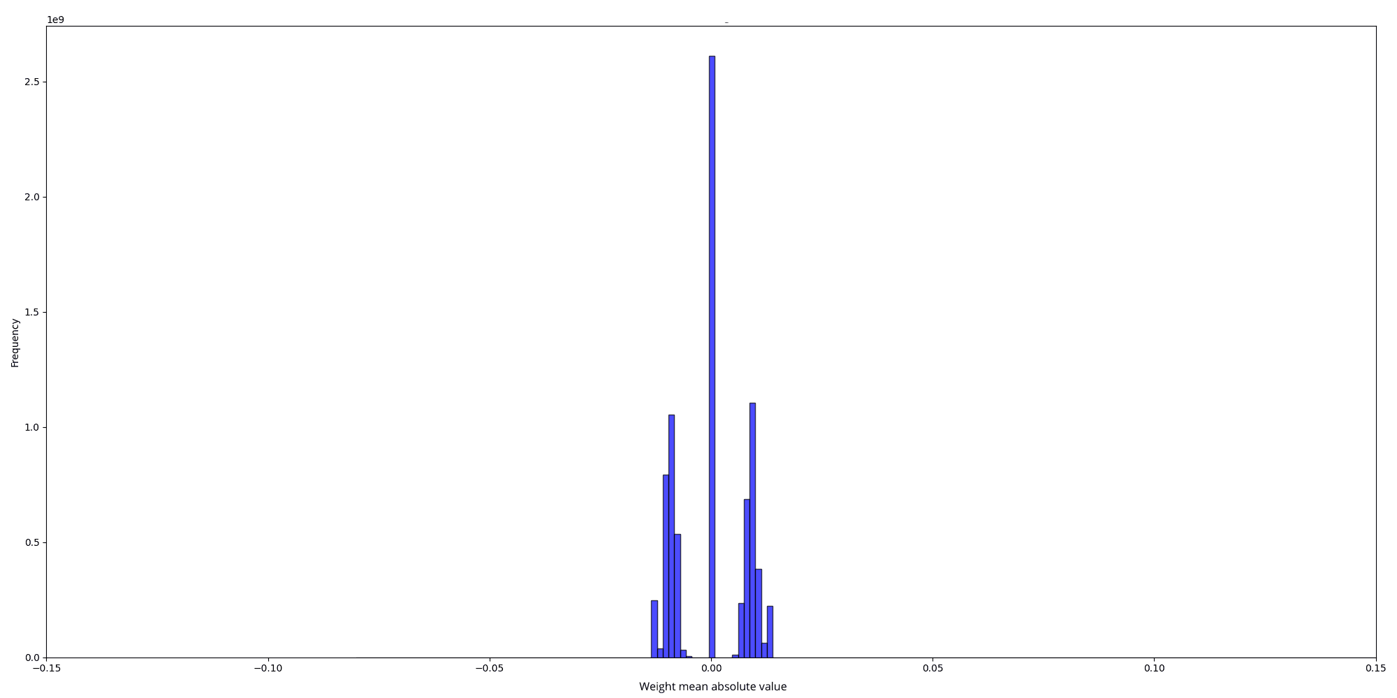
On the other hand, the pretrained weight's distribution looks like a normal distribution with an std = 0.013 \text{std} = 0.013 std = 0.013

Clearly, the pretrained model starts with more information (scales), while the randomly initialized model starts with practically no information and adds to it over time. Our conclusion was that starting with random weights gives the model minimal initial information, enabling a gradual learning process, while during fine-tuning, the introduction of BitLinear layers overwhelms the model into losing all its prior information.

To improve the fine-tuning results, we tried different techniques. For example, instead of using per-tensor quantization, we tried per-row and per-column quantization to keep more information from the Llama 3 weights. We also tried to change the way the scale is computed: instead of just taking the mean absolute value of the weights as a scale, we take the mean absolute value of the outliers as a scale (an outlier value is a value that exceeds k*mean_absolute_value, where k is a constant we tried to vary in our experiments), but we didn’t notice big improvements.

def scale_outliers(tensor, threshold_factor=1):
    mean_absolute_value = torch.mean(torch.abs(tensor))
    threshold = threshold_factor * mean_absolute_value
    outliers = tensor[torch.abs(tensor) > threshold]
    mean_outlier_value = torch.mean(torch.abs(outliers))
    return mean_outlier_value

def weight_quant_scaling(w):
    scale = 1.0 / scale_outliers(w).clamp_(min=1e-5)
    quantized_weights = (w * scale).round().clamp_(-1, 1) / scale
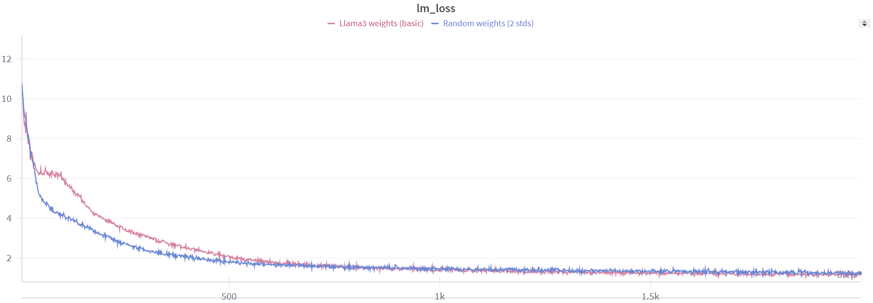
    return quantized_weights

We observed that both the random weights and the Llama 3 weights resulted in losses starting at approximately the same value of 13. This suggests that the Llama 3 model loses all of its prior information when quantization is introduced. To further investigate how much information the model loses during this process, we experimented with per-group quantization.

As a sanity check, we first set the group size to 1, which essentially means no quantization. In this scenario, the loss started at 1.45, same as we see during normal fine-tuning. However, when we increased the group size to 2, the loss jumped to around 11. This indicates that even with a minimal group size of 2, the model still loses nearly all of its information.

To address this issue, we considered the possibility of introducing quantization gradually rather than applying it abruptly to the weights and activations for each tensor. To achieve this, we implemented a lambda value to control the process :

lambda_ = ?
x_quant = x + lambda_ * (activation_quant(x) - x).detach()
w_quant = w + lambda_ * (weight_quant(w) - w).detach()

When lambda is set to 0, there is essentially no quantization occurring, while at lambda=1 , full quantization is applied.

We initially tested some discrete lambda values, such as 0.25, 0.5, 0.75, and 1. However, this approach did not lead to any significant improvement in results, mainly because lambda=0.25 is already high enough for the loss to start very high.

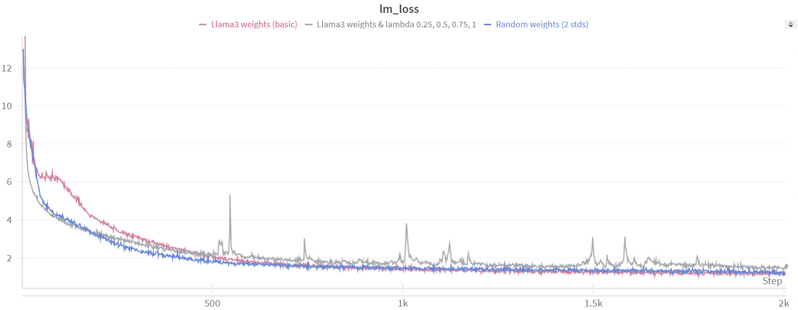
As a result, we decided to experiment with a lambda value that adjusts dynamically based on the training step.

lambda_ = training_step / total_training_steps

Using this dynamic lambda value led to better loss convergence, but the perplexity (ppl) results during inference, when lambda was set to 1, were still far from satisfactory. We realized this was likely because the model hadn't been trained long enough with lambda=1 . To address this, we adjusted our lambda value to improve the training process.

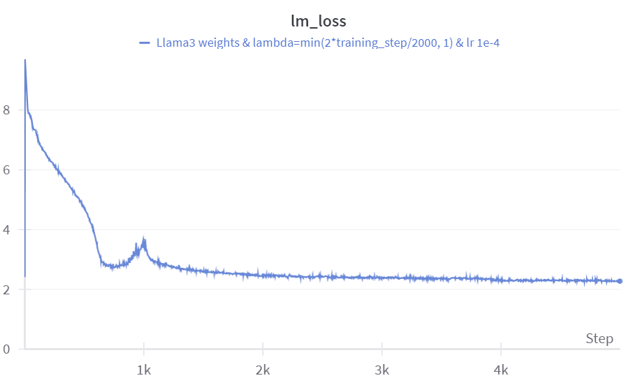
lambda_ = min(2 * training_step / total_training_steps, 1)

With this configuration, after 2000 steps we have :

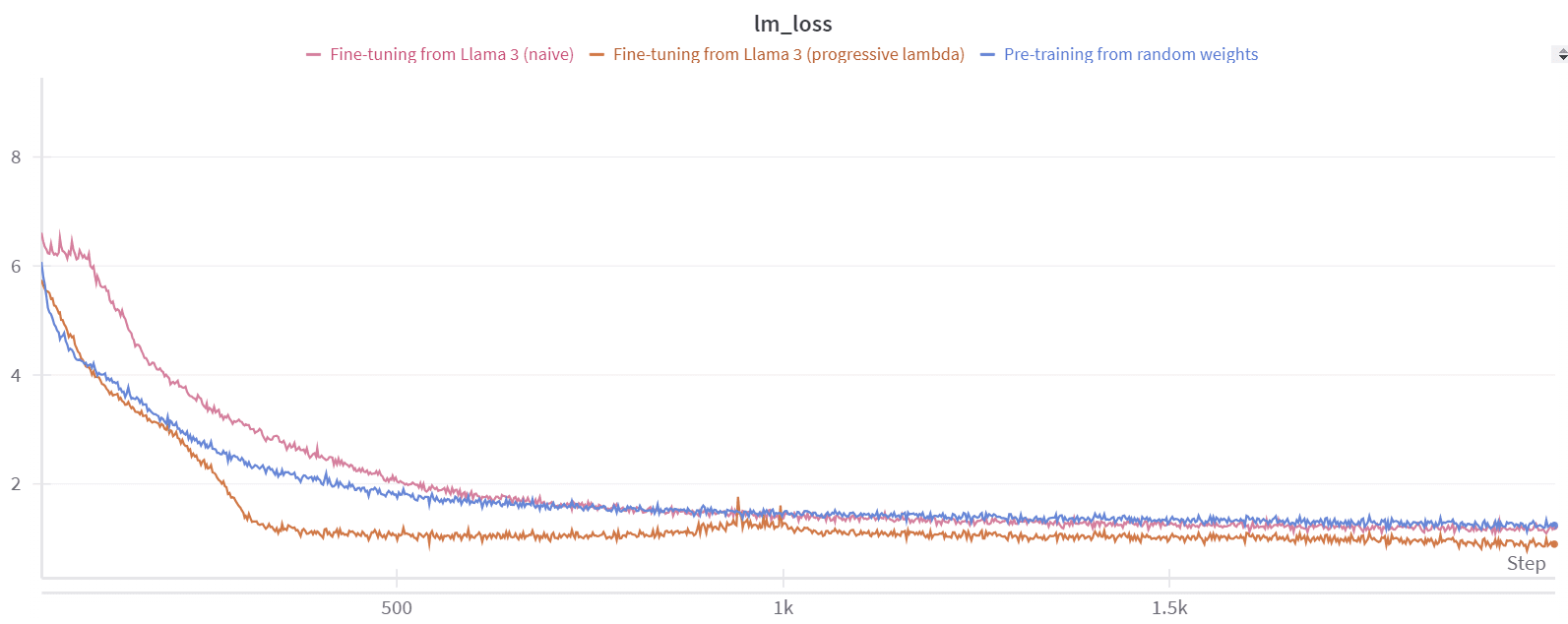
Our fine-tuning method shows better convergence overall. You can observe a slight increase in the loss curve around 1,000 steps, which corresponds to when we begin approaching lambda=1 , or full quantization. However, immediately after this point, the loss starts to converge again, leading to an improved perplexity of approximately 4.

Despite this progress, when we tested the quantized model on the WikiText dataset (instead of the tinystories one we used for fine-tuning), it showed a very high perplexity. This suggests that fine-tuning the model in low-bit mode on a specific dataset causes it to lose much of its general knowledge. This issue might arise because the minimal representations we aim for with ternary weights can vary significantly from one dataset to another. To address this problem, we scaled our training process to include the larger FineWeb-edu dataset. We maintained a lambda value of:

lambda_ = min(training_step/1000, 1)

We chose this lambda value because it seemed to be a good starting point for warming up the model. We then trained the model using a learning rate of 1e-4 for 5,000 steps on the FineWeb-edu dataset. The training involved a batch size (BS) of 2 million, totaling 10 billion tokens.

Finding the right learning rate and the right decay was challenging; it seems to be a crucial factor in the model's performance.

After the fine-tuning process on Fineweb-Edu, the perplexity on the WikiText dataset reached 12.2, which is quite impressive given that we only used 10 billion tokens. The other evaluation metrics also show strong performance considering the limited amount of data (see results).

We also tried to smooth out the sharp increase when lambda approaches 1. To do this, we considered using lambda schedulers that grow exponentially at first, then level off as they get closer to 1.

def scheduler(step, total_steps, k):
    normalized_step = step / total_steps
    return 1 - (1 - normalized_step)**k

for different k values, with a number of total warmup steps of 1, we have plots like the following :

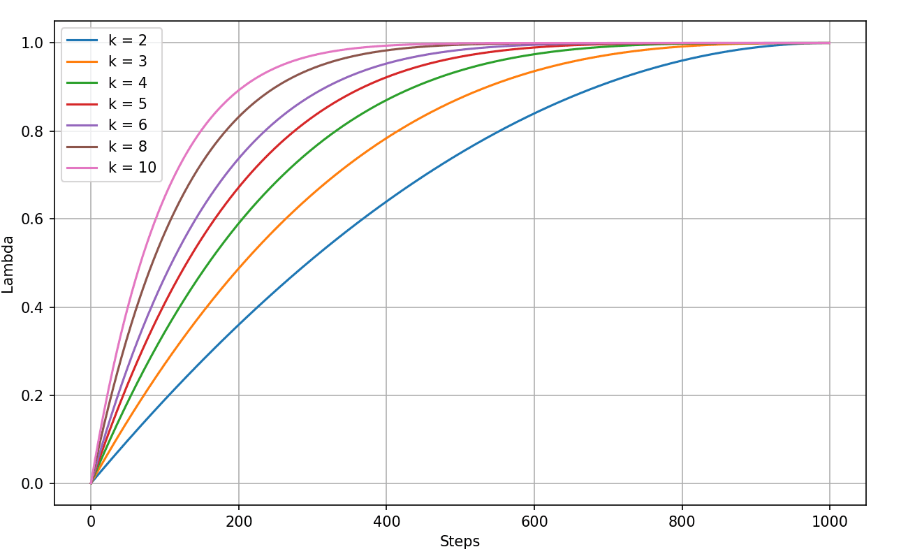
We ran 4 experiments using the best-performing learning rate of 1e-4, testing values of k in [4, 6, 8, 10].

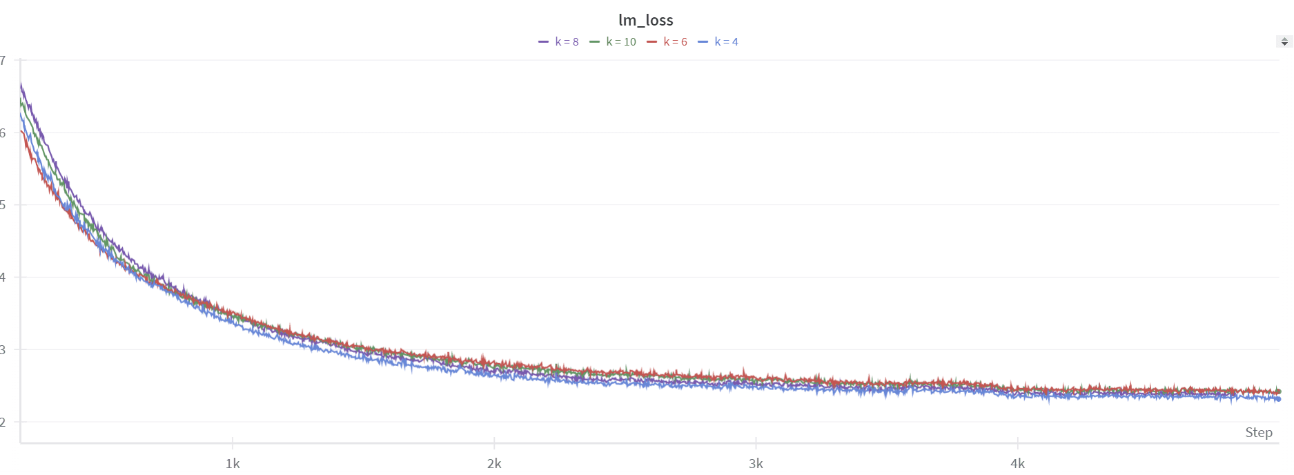
The smoothing worked well, as there's no spike like with the linear scheduler. However, the perplexity isn't great, staying around ~15, and the performance on downstream tasks is not better.

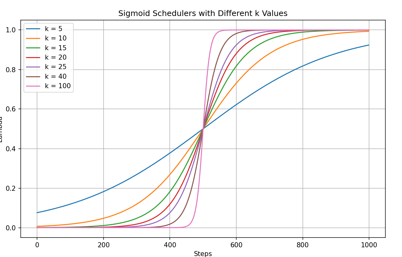
We also noticed the spike at the beginning, which the model struggled to recover from. With lambda = 0, there's essentially no quantization, so the loss starts low, around ~2. But right after the first step, there's a spike, similar to what happened with the linear scheduler (as seen in the blue plot above). So, we tried a different scheduler—a sigmoid one—that starts slowly, rises sharply to 1, and then levels off as it approaches 1.

def sigmoid_scheduler(step, total_steps, k):
    # Sigmoid-like curve: slow start, fast middle, slow end
    normalized_step = step / total_steps
    return 1 / (1 + np.exp(-k * (normalized_step - 0.5)))

For different k values we have the following curves :